There is only one test 🃏

Permutation, the bootstrap, and what a p-value actually says

All of hypothesis testing is one idea: build a world where nothing is going on, simulate it, and ask if your data would be surprising there. Learn it by shuffling with the tidyverse, then industrialize it with infer.

“To consult the statistician after an experiment is finished is often merely to ask him to conduct a post mortem examination. He can perhaps say what the experiment died of.”
–Ronald A. Fisher

PART I: One idea wearing twenty names

Open any statistics textbook and you find a zoo: t-tests, chi-squared tests, ANOVA, Mann-Whitney, each with its own formula, table and existence conditions. Here is the secret the zoo hides¹: they are all the same test, and you already have the tools to run it, because the previous session taught you to simulate sampling distributions.

The one test:

1. Compute a statistic from your data –a difference in means, a correlation, anything.
2. Build a null world: a version of reality where the effect you’re testing does not exist.
3. Simulate that world many times, computing the same statistic each time.
4. Ask: where does my real statistic fall in that distribution of nothing-going-on?

If your number sits comfortably in the middle of what nothing-going-on produces, you have learned nothing. If it sits in the far tail, the boring explanation strains –that tail probability is the infamous p-value.

Let’s run it on real penguins, imported straight from the web as this workshop likes it:

library(tidyverse)

penguins_raw <- readr::read_csv(
  "https://raw.githubusercontent.com/allisonhorst/palmerpenguins/main/inst/extdata/penguins.csv"
  )

penguins <- penguins_raw |>
  dplyr::filter(species != "Gentoo", !is.na(bill_length_mm)) |>
  dplyr::select(species, bill_length_mm)

penguins |>
  dplyr::summarise(mean_bill = mean(bill_length_mm), n = dplyr::n(), .by = species)

1

Two species, one question: do Adelie and Chinstrap penguins really differ in bill length, or could a gap like this arise from sampling noise?

# A tibble: 2 × 3
  species   mean_bill     n
  <chr>         <dbl> <int>
1 Adelie         38.8   151
2 Chinstrap      48.8    68

PART II: The permutation test, by hand

Our statistic is the difference in mean bill length:

observed_diff <- penguins |>
  dplyr::summarise(m = mean(bill_length_mm), .by = species) |>
  dplyr::summarise(diff = m[species == "Chinstrap"] - m[species == "Adelie"]) |>
  dplyr::pull(diff)

observed_diff

[1] 10.04243

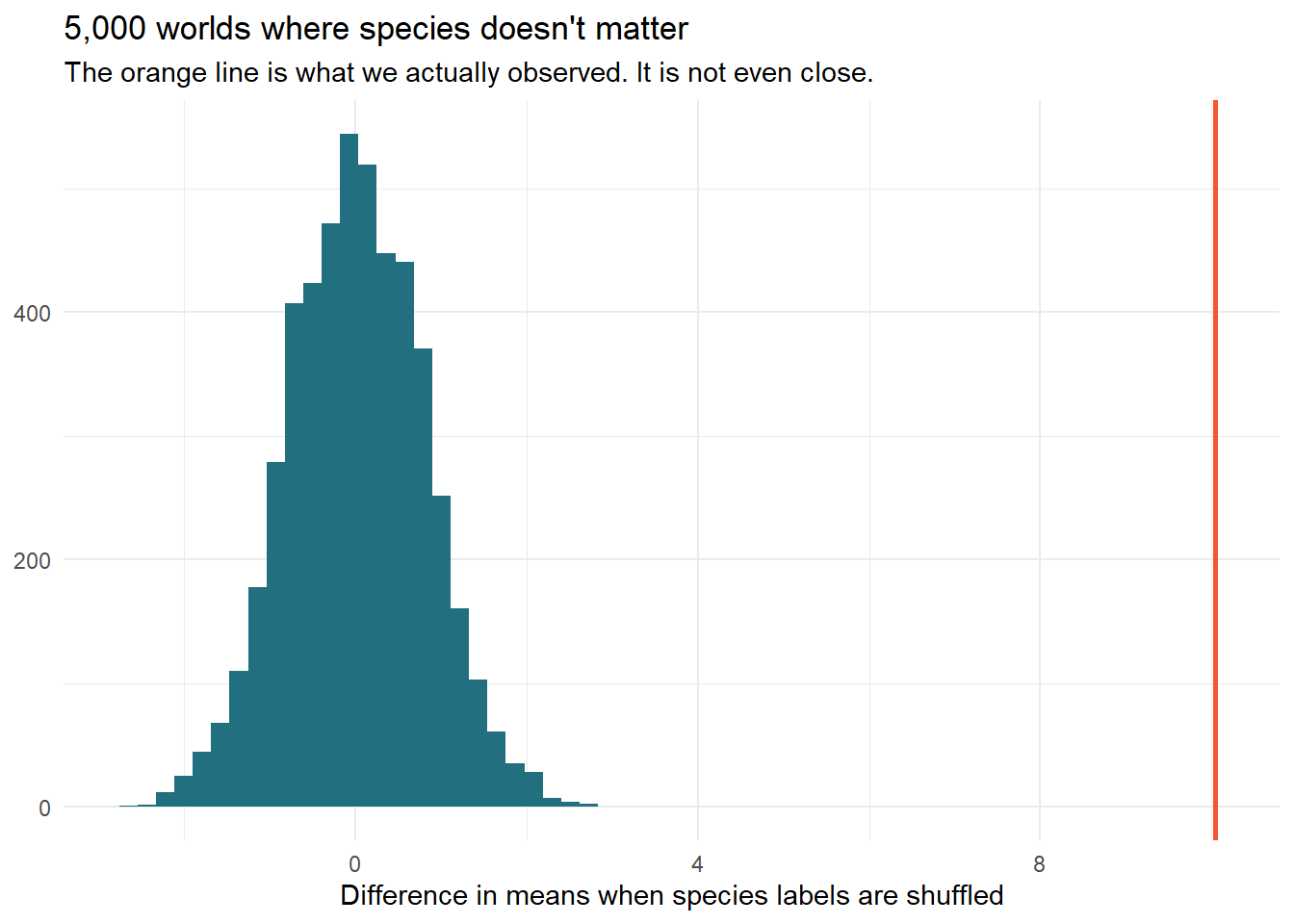
Now the null world. If species had nothing to do with bill length, the species labels would be arbitrary stickers –so we can build that world by shuffling the stickers and leaving the bills alone:

set.seed(2024)

null_world <- tibble(replicate = 1:5000) |>
  dplyr::mutate(
    diff = purrr::map_dbl(replicate, \(i) {
      penguins |>
        dplyr::mutate(species = sample(species)) |>
        dplyr::summarise(m = mean(bill_length_mm), .by = species) |>
        dplyr::summarise(d = m[species == "Chinstrap"] - m[species == "Adelie"]) |>
        dplyr::pull(d)
      })
    )

null_world |>
  ggplot(aes(diff)) +
  geom_histogram(bins = 60, fill = "#226F7F") +
  geom_vline(xintercept = observed_diff, color = "#F75431", linewidth = 1) +
  labs(
    x = "Difference in means when species labels are shuffled",
    y = NULL,
    title = "5,000 worlds where species doesn't matter",
    subtitle = "The orange line is what we actually observed. It is not even close."
    ) +
  theme_minimal()

1

sample(species) with no other arguments shuffles the column –every penguin keeps its bill, gets a random label. This single line is the null hypothesis, written in R instead of Greek.

The verdict needs no formula: in 5,000 label-shuffled worlds, the biggest difference noise ever produced is a fraction of what we observed. The p-value is the share of null worlds at least as extreme as reality:

mean(abs(null_world$diff) >= abs(observed_diff))

[1] 0

Zero out of 5,000². A t-test would have told you the same thing through a formula –now you know what the formula is estimating.

PART III: The same machine, industrialized –infer

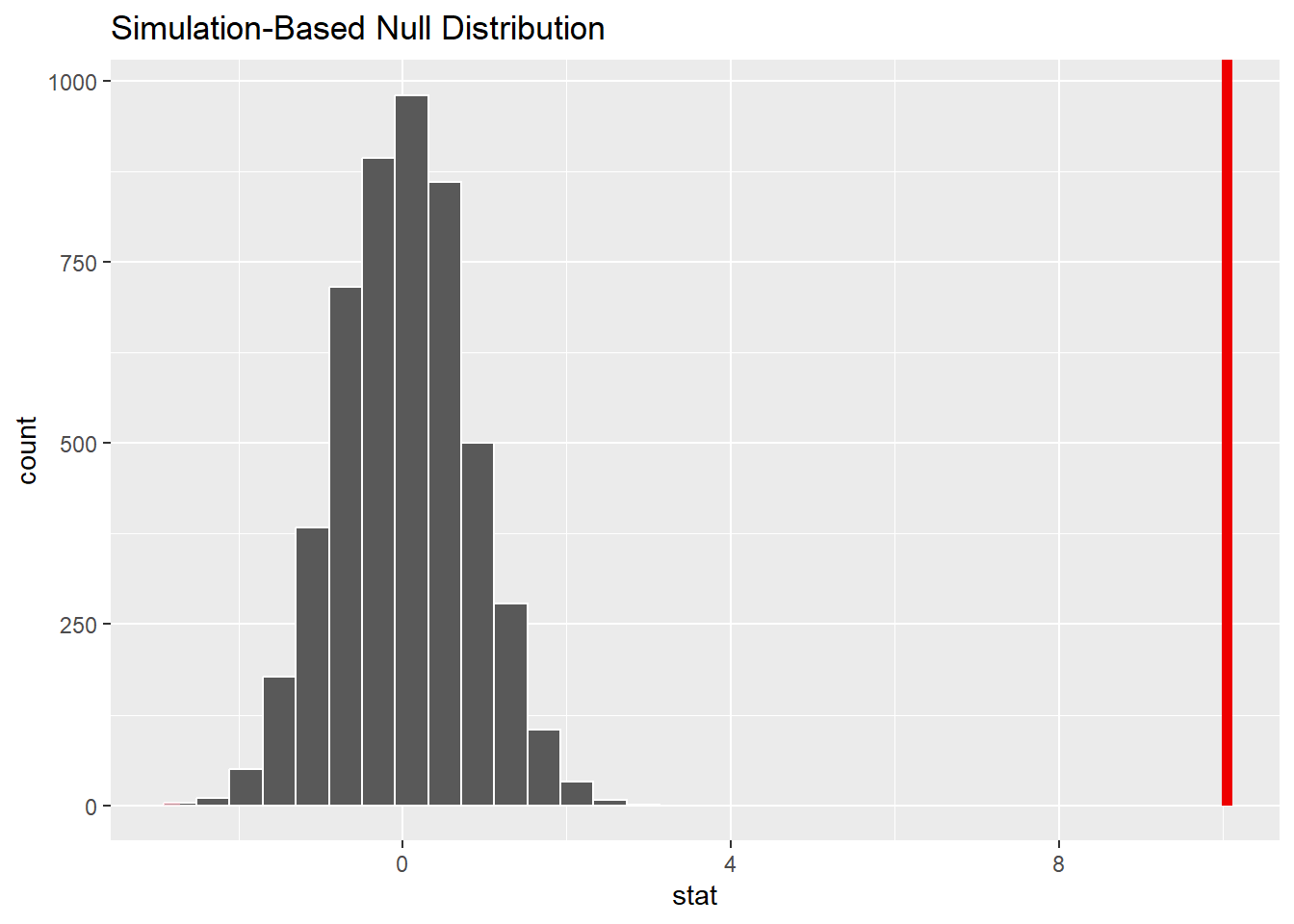
The infer package (tidymodels family) turns the four steps into four verbs –specify(), hypothesize(), generate(), calculate()– so the code reads like the logic:

library(infer)
set.seed(2024)

null_dist <- penguins |>
  infer::specify(bill_length_mm ~ species) |>
  infer::hypothesize(null = "independence") |>
  infer::generate(reps = 5000, type = "permute") |>
  infer::calculate(stat = "diff in means",
                   order = c("Chinstrap", "Adelie"))

null_dist |>
  infer::visualize() +
  infer::shade_p_value(obs_stat = observed_diff, direction = "two-sided")

1

The statistic’s recipe: outcome ~ grouping.

2

The null world: species and bill length are independent.

3

Build it 5,000 times, by permutation –our shuffle, industrialized.

4

Which statistic to track. Change "diff in means" to "diff in medians", "t", "Chisq"… and you have replaced half the textbook zoo without learning a new formula.

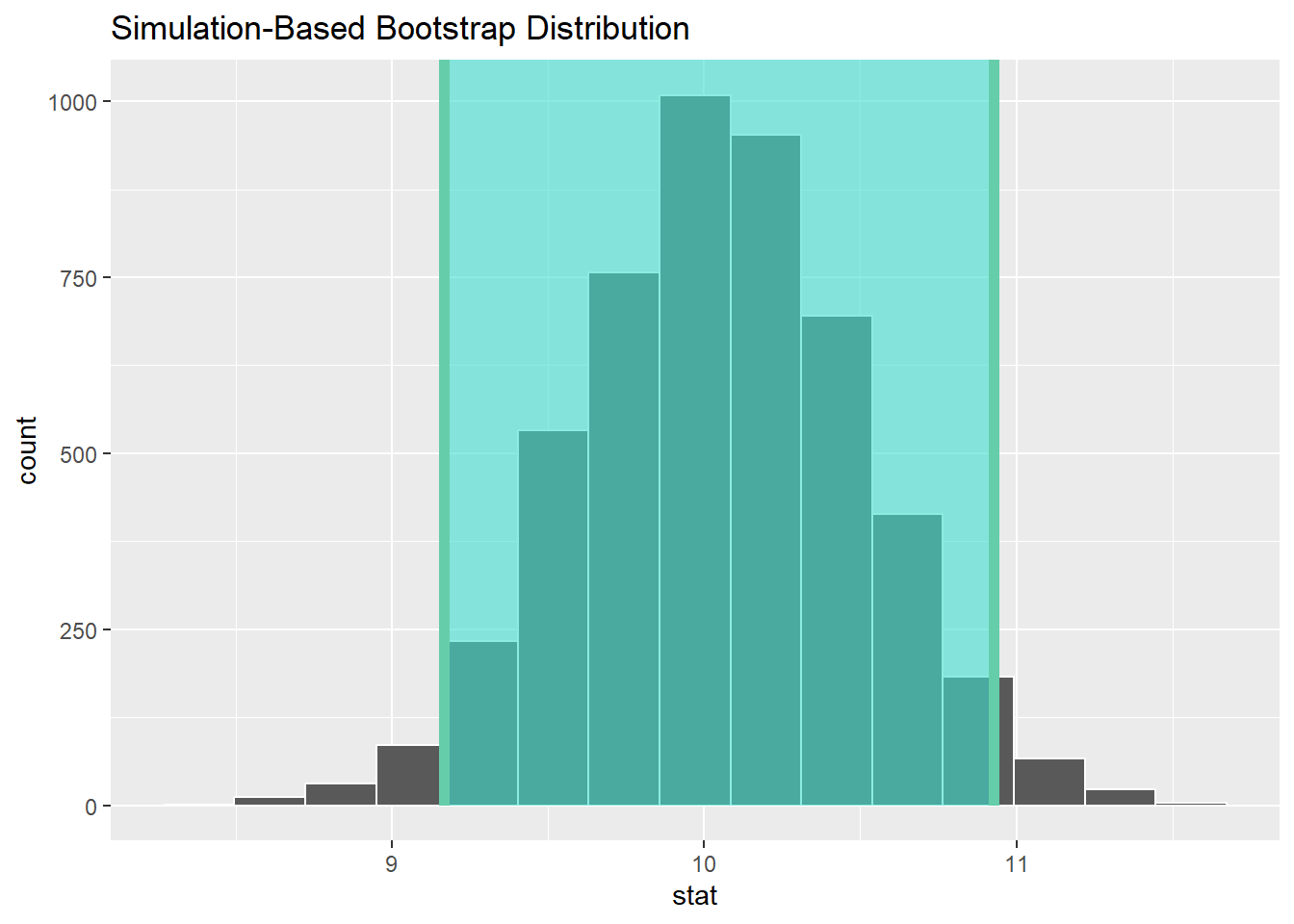
Bootstrap: the other side of the same coin

Permutation destroys a relationship to test it. The bootstrap does the reverse: it preserves the data and resamples it (with replacement) to measure how much your estimate wobbles –a confidence interval, without algebra:

set.seed(2024)

boot_dist <- penguins |>
  infer::specify(bill_length_mm ~ species) |>
  infer::generate(reps = 5000, type = "bootstrap") |>
  infer::calculate(stat = "diff in means",
                   order = c("Chinstrap", "Adelie"))

ci <- boot_dist |> infer::get_confidence_interval(level = 0.95)
ci

boot_dist |>
  infer::visualize() +
  infer::shade_confidence_interval(endpoints = ci)

1

Same pipeline, two changes: no hypothesize() (we’re estimating, not testing) and type = "bootstrap" (resample rows with replacement instead of shuffling labels).

# A tibble: 1 × 2
  lower_ci upper_ci
     <dbl>    <dbl>
1     9.17     10.9

Read it as: “if we could rerun this study endlessly, 95% of intervals built this way would capture the true difference.” Notice what the interval gives you that the p-value doesn’t: a magnitude with uncertainty, not just a verdict. Prefer it in almost every writeup.

PART IV: What the p-value is not

The p-value may be the most misquoted number in science, enough that the American Statistical Association issued a formal statement about it. Tattoo the correct reading somewhere: the probability of data at least this extreme, assuming nothing is going on. It is not:

• The probability the null hypothesis is true –that question needs Bayes, the last stop of this track.
• The probability the finding replicates.
• A measure of importance –with n large enough, a difference of 0.1mm in bill length becomes “significant” while mattering to no penguin.

And one misuse you can now demonstrate to yourself, rather than take on faith. Test twenty hypotheses where nothing –truly nothing– is going on:

set.seed(20)

tibble(experiment = 1:20) |>
  dplyr::mutate(
    p_value = purrr::map_dbl(experiment, \(i) {
      t.test(rnorm(30), rnorm(30))$p.value
      }),
    verdict = dplyr::if_else(p_value < 0.05, "SIGNIFICANT! 🎉", "ns")
    ) |>
  dplyr::filter(p_value < 0.05)

1

Both groups drawn from the same distribution: the null hypothesis is true by construction, twenty times. Yet significance arrives anyway –at 5% error per test, twenty tests make a false alarm more likely than not. This is the green jelly bean problem, and it is why “we tested many things and report the ones that worked” is not evidence, it’s arithmetic.

# A tibble: 1 × 3
  experiment p_value verdict                  
       <int>   <dbl> <chr>                    
1         17  0.0302 "SIGNIFICANT! \U0001f389"

WarningThe garden of forking paths

The jelly-bean trap doesn’t require running twenty literal tests. Choosing which outcome to measure, which subgroups to inspect, which observations count as outliers –each choice is a fork, and enough forks guarantee a “finding”. The defense is the discipline this workshop has preached from session 1: decide your analysis before looking, write it as code, version it. A committed script is a pre-registration you gave yourself.

TipExercises 🏋️

1. Rerun the permutation test with stat = "diff in medians". Does the conclusion survive a change of statistic? (Robust findings usually do.)
2. Use the full penguins data to test whether Gentoo and Adelie differ in flipper_length_mm, start to finish with infer.
3. Shrink the data: dplyr::slice_sample(n = 10, by = species) before the pipeline. What happens to the width of the bootstrap interval? Connect this to the \(\sqrt{n}\) rule from the previous session.
4. Simulate the forking-paths trap: generate one fake dataset with a null effect and 10 outcome variables; test all ten; report “the significant one”. Then explain, in one sentence, to your former self why this felt like science.

Next in the track: All models are wrong puts uncertainty inside the most-used model in the world –the regression line.

Footnotes

1. The framing is Allen Downey’s, from his classic post “There is still only one test”. The zoo of named tests exists because before computers, each special case needed its own hand-derivable algebra. You have a computer.

2. Which we honestly report as p < 1/5000, not p = 0 –our simulation just wasn’t big enough to see an event that rare.