- 1
-
Read the file into R with the function
pdf_text() - 2
- Eliminate all blank spaces in the text
Data from words 📚
Learn how to transform information stored in text as data you can analyse and visualise
text
sentiment
ngrams
pdf
book
network
regex
wordcloud
Import, clean, tokenise and stem text, plus do sentiment analysis, topic modelling and learn how functions in R make your work so much easier.
“For every complex problem there is an answer that is clear, simple, and wrong.”
–H.L. Mencken
Text analysis is how you convert prose into a numerical analysis. Examples of applications of text analysis are Google NGrams and translators like DeepL. It is also a building block for AI applications, like the recently released ChatGPT.
In this session we will focus on retrieving, cleaning and visualising text data.
Level: Intermediate · Time: ~90 min · Prerequisites: Everything in its right place · Tools: tidytext, stringr, dplyr, ggwordcloud, topicmodels
You will learn to
- Import text from a PDF and clean it into tidy, one-word-per-row data.
- Use regular expressions to find and remove patterns in text.
- Reduce words to stems and lemmas, and count what’s left.
- Score sentiment and build a wordcloud from word frequencies.
- Discover latent topics in a collection of documents with topic modelling.
PART I: Text to data
To get us started, we need to learn how to transform and clean text data. We’ll use an example of a book as a warm up.
Breaking down “The Origin of Species”
We’ll use Charles Darwin’s “On the Origin of Species by Means of Natural Selection, or the Preservation of Favoured Races in the Struggle for Life” to illustrate how to go from text to data.
We first download a PDF copy of the book online (like this one). Then, using the pdftools package, we can import the text into R. PDF is a terrible format to store data, you’ll see why soon.
TipRegular expressions, regex
Regular expressions are a way to specify or search for patterns of strings using a sequence of characters. By combining a selection of simple patterns, we can capture quite complicated combinations of strings.
Read this appendix of Supervised Machine Learning for Text Analysis in R and use regexr to learn how to draw the text data you need using regular expressions
Working with text-as-data: Tokenization, stopwords, stemming
Before we can actually use the text to analyse it, we need to perform a few operations. The first is to create tokens, which is basically the unit of measurement we choose for our text analysis. Token can be words, characters, sentences, paragraphs, n-grams, you name it. To tokenize the book, we’ll use a function from the tidytext package that does all the heavy lifting for us.
TipA sliver of regex
regex gives headaches, and the 2nd page of the stringr cheatsheet is your ibuprofen. There are a few important operations in regex you should remember:
Special metacharacters
\.Represents a period. To match a period, type\\.\\Represents a single backslash. To match two backslashes, type\\\\\"Represents a single quotation sign.\nNew line
Anchors
^Start of the string$End of the string\\bEmpty string at either edge of a word
Stop! Removing words we don’t care much about
We will then extract words from the remaining data that we won’t need. These are called stopwords, and include a list of articles, prepositions and other words that we are not super interested in analysing. We will remove the words using the anti_join() function, which removes any common elements from two databases.
Looking for the root and a bit of linguistics
Finally, we will look at the stem of the remaining words, as we want to avoid duplicates from plurals and the like. For this we will use the SnowballC package, which has a handy function to extract the root of words. We also do lemmatization, or identifying the dictionary form of the words based on linguistics and grouping them together using the textstem package.
We won’t go into the details, but check the differences between the stem and lemma results below to pick your curiosity:
library(pdftools)
library(tidytext)
library(tidyverse)
library(hunspell)
library(SnowballC)
library(textstem)

# Tokenization - Turn all text into a data frame of words ####
toos_df <- the_origins_of_species |>
3  tibble::as_tibble() |>
4  tidytext::unnest_tokens(input = "value", output = "word", token = "words", to_lower = TRUE)

# Stopwords - Remove them with anti_join ####
5stopwords::stopwords(language = "en")

# Now let's remove all the stop words from our data and stem the text ####
toos_df |>
6  dplyr::anti_join(stopwords::stopwords(language = "en") |>
                     as_tibble(),
                   by=c("word"="value")) |>
7  dplyr::mutate(stem = SnowballC::wordStem(word),
lemma = textstem::lemmatize_words(word))- 3
- Make into a database
- 4
-
Tokenize into words using the
unnest_tokens()function. We also make the text lower-case. - 5
- See the list of stopwords in each language
- 6
-
Remove all the stopwords from the list using
anti_join(), which removes all words common in both datasets. - 7
- Identify the stem of each word, to avoid counting conjugation duplicates, and lemmatization that uses linguistics to create lemmas, the canonical or dictionary forms of word.
  [1] "i"          "me"         "my"         "myself"     "we"
  [6] "our"        "ours"       "ourselves"  "you"        "your"
 [11] "yours"      "yourself"   "yourselves" "he"         "him"
 [16] "his"        "himself"    "she"        "her"        "hers"
 [21] "herself"    "it"         "its"        "itself"     "they"
 [26] "them"       "their"      "theirs"     "themselves" "what"
 [31] "which"      "who"        "whom"       "this"       "that"
 [36] "these"      "those"      "am"         "is"         "are"
 [41] "was"        "were"       "be"         "been"       "being"
 [46] "have"       "has"        "had"        "having"     "do"
 [51] "does"       "did"        "doing"      "would"      "should"
 [56] "could"      "ought"      "i'm"        "you're"     "he's"
 [61] "she's"      "it's"       "we're"      "they're"    "i've"
 [66] "you've"     "we've"      "they've"    "i'd"        "you'd"
 [71] "he'd"       "she'd"      "we'd"       "they'd"     "i'll"
 [76] "you'll"     "he'll"      "she'll"     "we'll"      "they'll"
 [81] "isn't"      "aren't"     "wasn't"     "weren't"    "hasn't"
 [86] "haven't"    "hadn't"     "doesn't"    "don't"      "didn't"
 [91] "won't"      "wouldn't"   "shan't"     "shouldn't"  "can't"
 [96] "cannot"     "couldn't"   "mustn't"    "let's"      "that's"
[101] "who's"      "what's"     "here's"     "there's"    "when's"
[106] "where's"    "why's"      "how's"      "a"          "an"
[111] "the"        "and"        "but"        "if"         "or"
[116] "because"    "as"         "until"      "while"      "of"
[121] "at"         "by"         "for"        "with"       "about"
[126] "against"    "between"    "into"       "through"    "during"
[131] "before"     "after"      "above"      "below"      "to"
[136] "from"       "up"         "down"       "in"         "out"
[141] "on"         "off"        "over"       "under"      "again"
[146] "further"    "then"       "once"       "here"       "there"
[151] "when"       "where"      "why"        "how"        "all"
[156] "any"        "both"       "each"       "few"        "more"
[161] "most"       "other"      "some"       "such"       "no"
[166] "nor"        "not"        "only"       "own"        "same"
[171] "so"         "than"       "too"        "very"       "will"
# A tibble: 111,883 × 3
   word     stem     lemma
   <chr>    <chr>    <chr>
 1 charles  charl    charles
 2 robert   robert   robert
 3 darwin   darwin   darwin
 4 frs      fr       frs
 5 frgs     frg      frgs
 6 fls      fl       fls
 7 fzs      fz       fzs
 8 ˈdɑːrwɪn ˈdɑːrwɪn ˈdɑːrwɪn
 9 12       12       12
10 february februari february
# ℹ 111,873 more rows
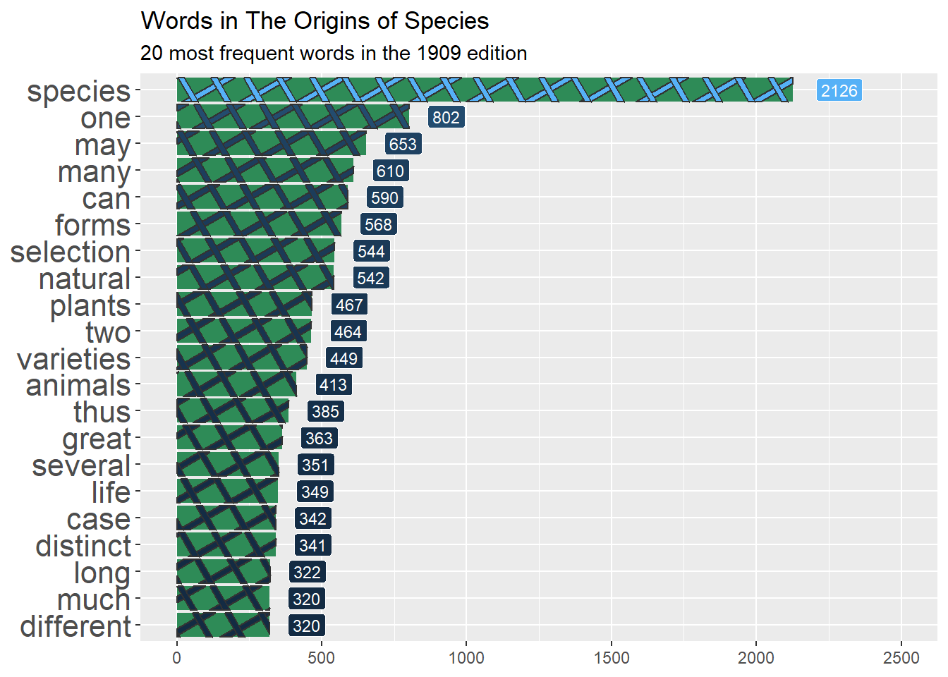
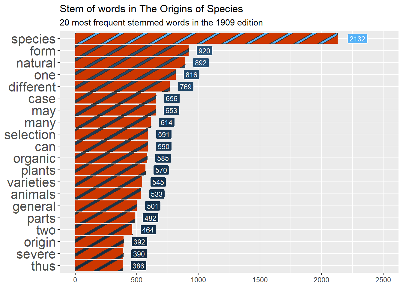
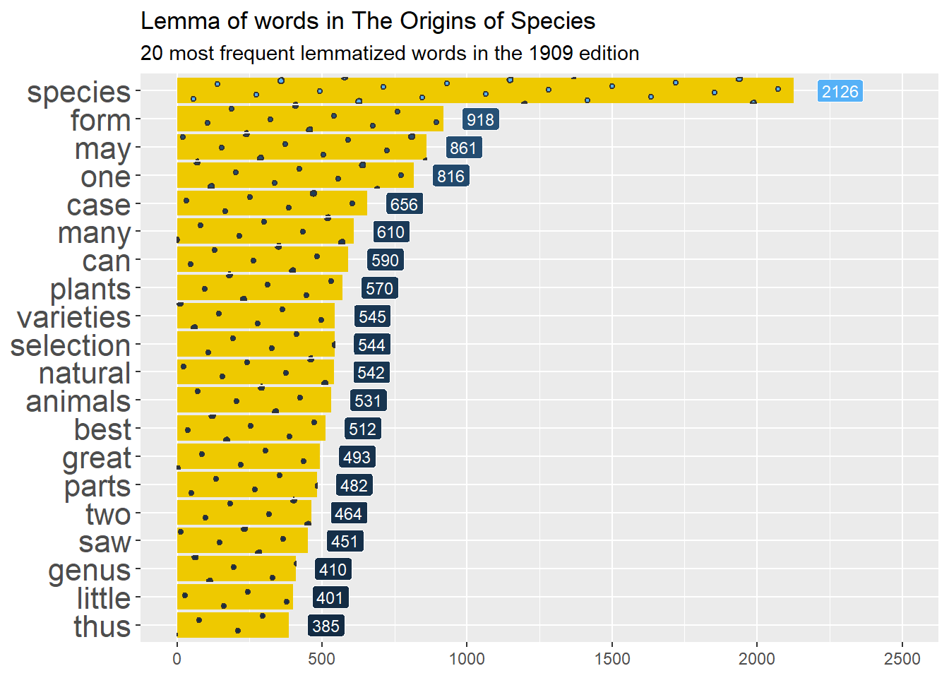
Now let’s see the result from the cleaning by plotting the frequency of the words that appear the most in the book using ggplot2 –for words, their stems and also their lemmas. We will start with the original data and, using the pipe, clean it, sort it, slice it and feed it to ggplot. In this case, we want bars/columns to represent the frequency of each word. We’ll use the package ggpattern to style the bars, so we use geom_col_pattern() with pattern options, and geom_label() to add the numeric frequency of the word next to each bar.
Compare the results below, and notice the differences:
Wordclouds with ggwordcloud
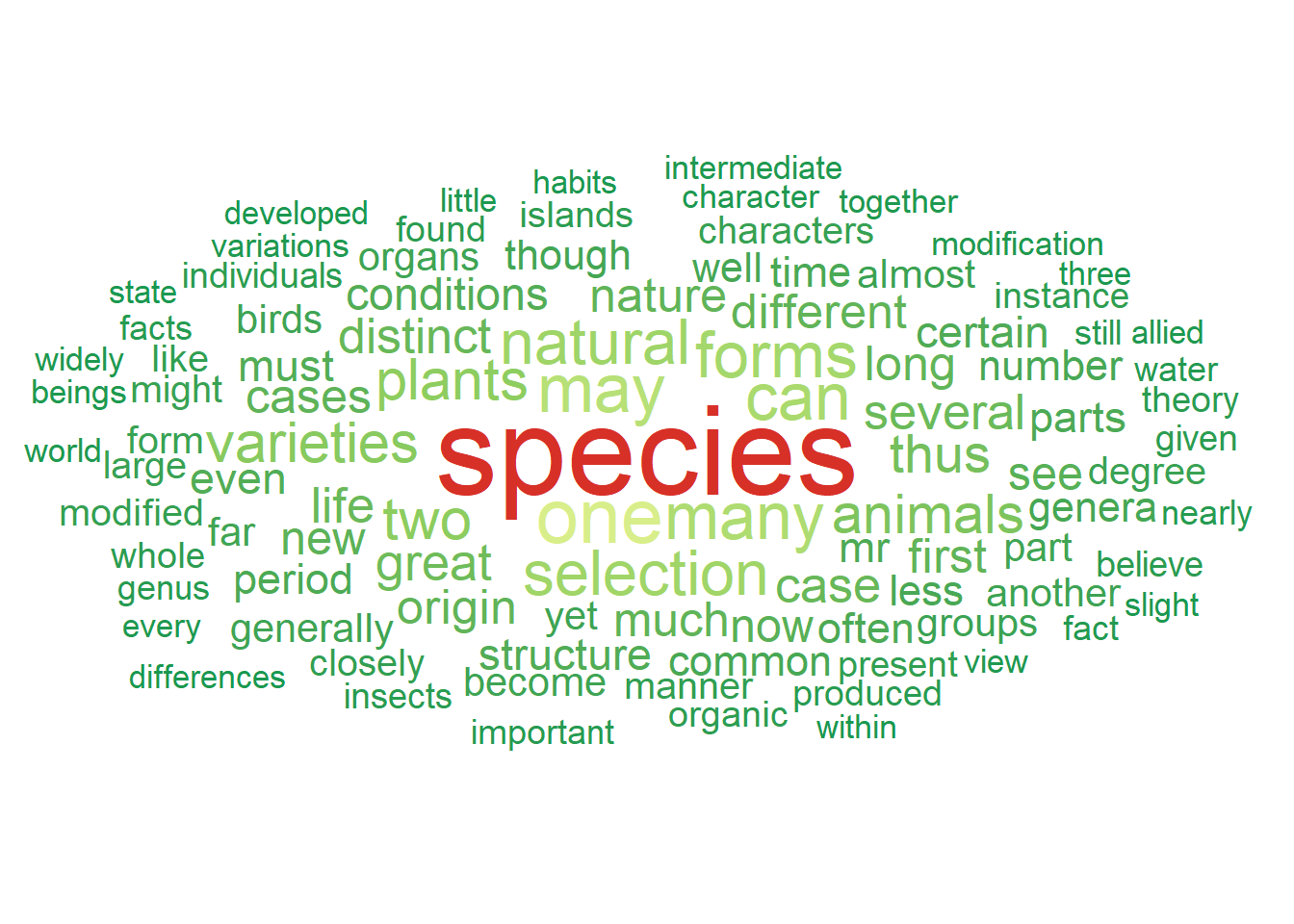
Wordclouds are mostly decorative, they are not very informative. They are the pie charts of text data: There will always be a better way to convey the information, but people like them anyway.
To create a wordcloud, we only need to use one new geometry: geom_text_wordcloud(). As arguments we give the label for each word and the weight of the word based on the frequency. we can also change the area in which the wordcloud is created, using the scale_size_area() option and a 3-color diverging palette.
library(tidyverse)
library(ggwordcloud)
library(RColorBrewer)

toos_df |>
  dplyr::anti_join(stopwords::stopwords(language = "en") |>
                     as_tibble(), by=c("word"="value")) |>
  dplyr::group_by(word) |>
  dplyr::summarise(word_count = n()) |>
  dplyr::distinct(word, .keep_all = TRUE) |>
  dplyr::slice_max(order_by=word_count, n = 100) |>
  ggplot()+
8  ggwordcloud::geom_text_wordcloud(aes(label = word, size = word_count, color=word_count)) +
  scale_size_area(max_size = 17) +
  scale_color_distiller(palette="RdYlGn", direction=-1)+
theme_minimal()- 8
-
Use the
geom_text_wordcloud()geometry to plot the wordcloud very easily, even adding a variable to weight the size by frequency in the text and color it with a palette.
Sentiment analysis for Infinite Jest
Words have connotations that can be analysed numerically. Evaluating an opinion or emotion in text can be done using sentiment analysis, which we will do for another american novel: David Foster Wallace’s Infinite Jest. To do this, we just need to add a database with negative/positive identifiers for words in English and match them with the data from the book.
We’ll use the lexicon Bing to start, which gives either a single positive or negative association to a large set of words in English.
library(textdata)
library(tidytext)

# Look at the list of words and +/- sentiment ####
tidytext::get_sentiments("bing")
# A tibble: 6,786 × 2
word sentiment
<chr> <chr>
1 2-faces negative
2 abnormal negative
3 abolish negative
4 abominable negative
5 abominably negative
6 abominate negative
7 abomination negative
8 abort negative
9 aborted negative
10 aborts negative
# ℹ 6,776 more rowsWith the pipe workflow, we sequence all the steps we did before and join the sentiment lexicon to get a visual summary of the frequency of positive or negative words in this mammoth novel.
Tip
dplyr helper functions
The dplyr package has some useful functions that regex text without a hassle: you can select variables or filter observations based on text.
starts_with: starts with a prefix (same as regex ‘^blah’)ends_with: ends with a prefix (same as regex ‘blah$’)contains: contains a literal string (same as regex ‘blah’)matches: matches a regular expression (write regex here)num_range: a numerical range like x01, x02, x03 (same as regex ‘x[0-9][0-9]’)one_of: variables in character vectoreverything: all variables. Used for reordering.
library(textdata)
library(RColorBrewer)
library(tidyverse)
library(tidytext)

9pdftools::pdf_text(paste0(getwd(),"/infinite_jest.pdf")) |>
10  stringr::str_squish() |>
11  tibble::as_tibble() |>
12  tidytext::unnest_tokens(input = "value", output = "word", token = "words") |>
13  dplyr::anti_join(stopwords::stopwords(language = "en") |>
                     as_tibble(), by=c("word"="value")) |>
14  dplyr::left_join(get_sentiments("bing"),
                   by=c("word")) |>
15  dplyr::filter(!is.na(sentiment)) |>
16  dplyr::group_by(sentiment) |>
  dplyr::summarise(sentiment_count = n()) |>
  # Plot
17  ggplot(aes(x=sentiment,y=sentiment_count,fill=sentiment))+
  geom_col(show.legend = FALSE)+
  coord_flip()+
  labs(x=NULL,y="Word count",
       title = "Infinite Jest by David Foster Wallace",
       subtitle = "Text analysis using Bing")+
scale_fill_manual(values = c("blue","red"))- 9
-
Import the book into R with
pdf_text(), which returns one character string per page. - 10
-
Collapse repeated whitespace and line breaks into single spaces with
str_squish(). - 11
- Turn the character vector into a tibble, the rectangular shape the rest of the pipeline expects.
- 12
-
Tokenize:
unnest_tokens()breaks each page into one row per word, lowercased. - 13
-
Remove stopwords (“the”, “and”, “of”…) with
anti_join(): keep only the words that do not appear in the stopword list. - 14
-
Attach a sentiment to every word that has one, joining against the Bing lexicon with
left_join(). - 15
-
Words absent from the lexicon came back as
NA–filter them out. - 16
- Group and summarise the count of words by sentiment.
- 17
-
Pipe the summary straight into
ggplot–no intermediate object needed.
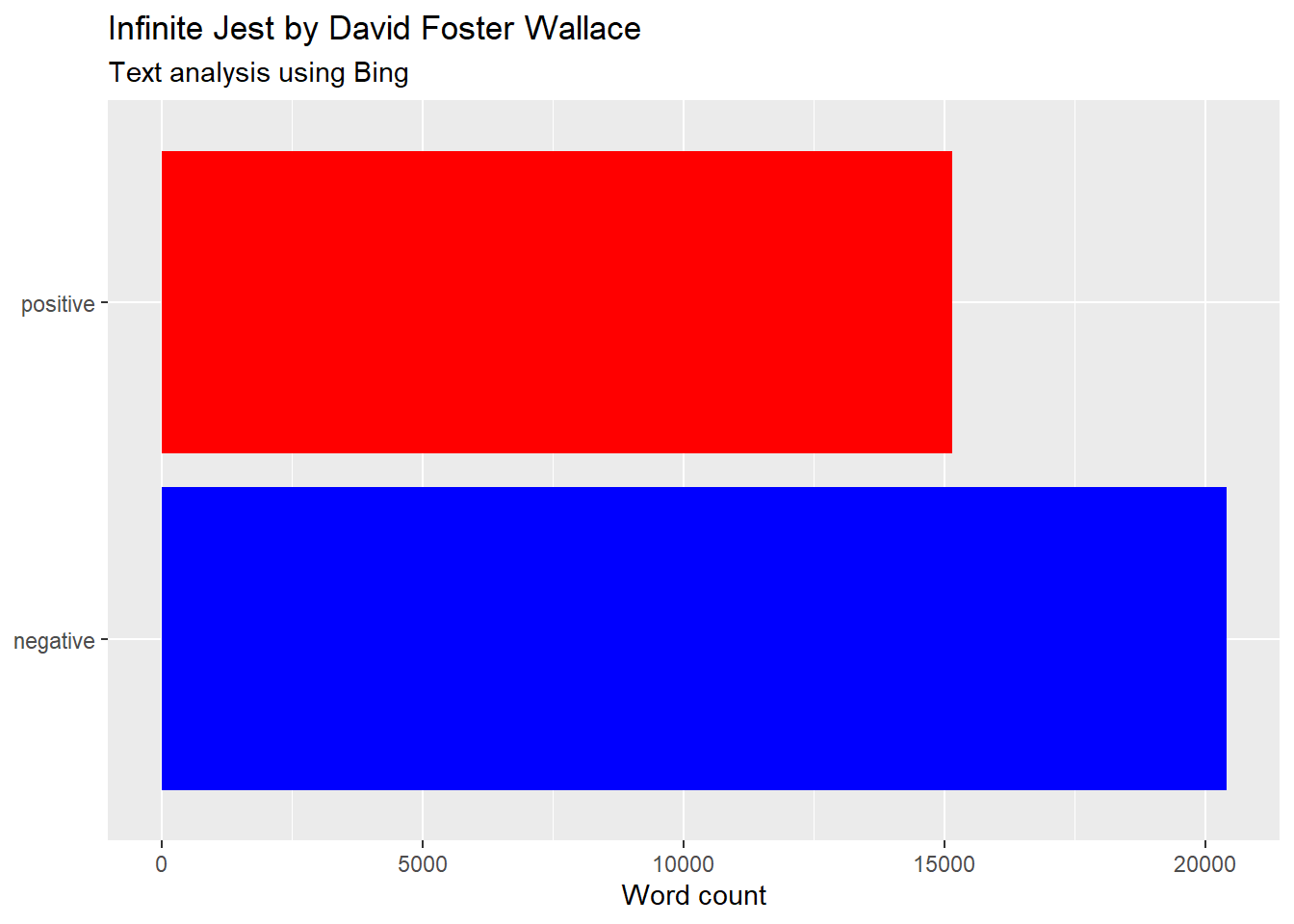
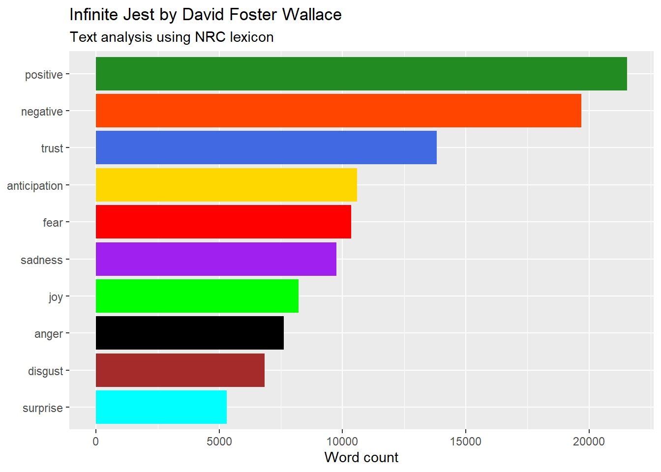
The positive/negative lexicon is not very interesting. There is another one called NRC1 which is more nuanced.
Let’s repeat the analysis using this lexicon and draw word frequencies by sentiment group, taking into account that words can have multiple sentiments and will be counted multiple times. Using scale_fill_manual() we can easily assign a color to each sentiment.
TipJoin us! Merging data with
dplyr
Merging data between databases using dplyr is a joy, not a headache. There are several join functions that ease combining datasets based on common variables:
inner_join()returns only the matching rows from both datasets, keeping only the observations with common values in the specified variables.left_join()returns all rows from the left dataset and the matching rows from the right dataset, keeping all observations from the left dataset and only the matching ones from the right dataset.right_join()is similar to left_join(), but it keeps all observations from the right dataset and only the matching ones from the left dataset.full_join()returns all rows from both datasets, keeping all observations from both datasets and filling in missing values with NAs when there is no match.semi_join()returns only the rows from the left dataset that have a match in the right dataset, discarding observations without a match.anti_join()returns all rows from the left dataset that do not have a match in the right dataset. It essentially removes the rows with matching values in the specified variables, keeping only the observations from the left dataset that have no corresponding match in the right dataset.
You can specify the columns for matching using the by argument within the chosen join function to specify the columns that should be used for matching. If you want to join based on a single column named “ID”, you would write: by = "ID". If you want to match on multiple columns, such as “ID” and “Date”, you would write: by = c("ID", "Date")).
library(textdata)
library(RColorBrewer)
library(tidyverse)
library(tidytext)

# NRC lexicon ####
18nrc <- tidytext::get_sentiments("nrc")

# Import book ####
19pdftools::pdf_text(paste0(getwd(),"/infinite_jest.pdf")) |>
20  stringr::str_squish() |>
21  tibble::as_tibble() |>
22  tidytext::unnest_tokens(input = "value", output = "text", token = "words") |>
23  dplyr::anti_join(stopwords::stopwords(language = "en") |>
                     as_tibble(), by=c("text"="value")) |>
24  dplyr::left_join(nrc,
                   by=c("text"="word"), multiple="all") |>
25  dplyr::filter(!is.na(sentiment)) |>
26  dplyr::group_by(sentiment) |>
  dplyr::summarize(sentiment_count = n()) |>
  # Plot
  ggplot(aes(x=reorder(sentiment, sentiment_count), y=sentiment_count,fill=sentiment))+
  geom_col()+
  coord_flip()+
  labs(x=NULL,y="Word count",
       title = "Infinite Jest by David Foster Wallace",
       subtitle = "Text analysis using NRC lexicon")+
  theme(legend.position = "none")+
27  scale_fill_manual(values=c(
    "positive"="forestgreen",
    "negative"="orangered",
    "trust"="royalblue",
    "anticipation"="gold",
    "fear"="red",
    "sadness"="purple",
    "joy"="green",
    "anger"="black",
    "disgust"="brown",
    "surprise"="cyan")
)- 18
-
Retrieve the NRC sentiment lexicon with
get_sentiments(). Unlike Bing’s positive/negative pair, NRC maps words to ten sentiment categories. - 19
- Import the text into R, as before.
- 20
- Collapse repeated whitespace into single spaces.
- 21
- Turn the character vector into a tibble.
- 22
- Tokenize into one row per word.
- 23
-
Remove all stopwords using
anti_join(). - 24
-
Join the sentiments using
left_join(). A word can carry several NRC sentiments, so we addmultiple = "all"to keep every match, not just the first. - 25
- Filter out all words without a sentiment matched to them.
- 26
- Group and summarise the count of words by sentiment.
- 27
-
Notice how you can customise the colors using
scale_fill_manual(): a named vector of"value" = "color"pairs manually matches each sentiment to a color.
Rejoinder: Narrative progression in Moby Dick 🐋
A fun application of sentiment analysis is tracking the frequency of words by sentiment from beginning to end of a novel. We’ll use Moby Dick as an example, showing with the help of girafe, how the relative frequency of each sentiment in the Bing lexicon changes throughout the novel between positive and negative words.
As you can see below, the book grows progressively more negative, as the cumulative word count by sentiment shows.
library(gutenbergr)
library(tidytext)
library(tidyverse)
library(ggiraph)

moby_dick <- gutenbergr::gutenberg_works(title=="Moby Dick; Or, The Whale") |>
  gutenbergr::gutenberg_download(mirror = "http://mirrors.xmission.com/gutenberg/")

# Override and direct download
moby_dick <- readr::read_tsv("http://aleph.gutenberg.org/2/4/8/2489/2489-0.txt") |>
  tibble::as_tibble() |>
  dplyr::rename("text"=1)

moby_dick_gg <- moby_dick |>
  dplyr::mutate(chapter = cumsum(str_detect(text, regex("^chapter ", ignore_case = TRUE)))) |>
  dplyr::filter(chapter>0) |>
  tidytext::unnest_tokens(input = "text", output = "text", token = "words") |>
  dplyr::anti_join(stopwords::stopwords(language = "en") |>
                     as_tibble(), by=c("text"="value")) |>
  dplyr::left_join(tidytext::get_sentiments("bing"),
                   by=c("text"="word")) |>
  dplyr::filter(!is.na(sentiment)) |>
  dplyr::group_by(chapter, sentiment) |>
  dplyr::summarise(sent_chapter = n()) |>
  dplyr::group_by(sentiment) |>
  dplyr::mutate(cum_sent = cumsum(sent_chapter)) |>
  dplyr::group_by(chapter) |>
  dplyr::mutate(dif = (cum_sent - lag(cum_sent))) |>
  ggplot(aes(x=chapter))+
  geom_path_interactive(size = 3,
                        aes(y=cum_sent,
                            data_id = sentiment,
                            tooltip = sentiment,
                            color=sentiment))+
  geom_col_interactive(data = . %>% filter(!is.na(sentiment)),
                       fill="royalblue",
                       aes(y=dif,
                           data_id = sentiment,
                           tooltip = dif))+
  labs(x="Chapter",
       y="Cumulative count of words by sentiment")+
  theme_classic()+
  theme(legend.position = "top", legend.title = element_blank())+
  scale_color_manual(values=c(
    "positive"="forestgreen",
    "negative"="red2"
       )
    )

girafe(ggobj = moby_dick_gg,
       options = list(
         opts_hover_inv(css = "opacity:0.1;"),
         opts_tooltip(opacity = 0.8, css ="background-color:blue;color:white"),
         opts_zoom(max=4)
       )
)
PART II: Book shuffle using topic modelling2
A cool application of text analysis, topic modelling, tries to answer a very practical question: Take two or more texts. How are they related to one another?
Imagine the following situation. Someone scrambles all chapters of all OECD reports written over the past year, leaving thousands of files without names or any indication of which report they belong to. You know how many reports there were originally and are tasked to stitch back together all reports. How would you do that?
Using statistical techniques over text data pulled from all the scrambled chapters, you can try to infer how each leftover document is similar in style, content, word frequency and other features of the text to try to estimate how likely it is that 2 documents belong to the same report.
We’ll do exactly this but not over OECD reports, because that would be too boring. So we’ll do it over scrambled chapters from classical works of fiction and non-fiction.
Let’s first make a mess of some literature.
Choosing which books to shuffle
Project Gutenberg holds many works of literature that don’t have copyright anymore and are ready for text analysis. We’ll choose some books, download them into R using the gutenbergr package, and then break them apart by chapter in order to use topic modelling to stitch them back together.
These are the books we’ll use:
- The Picture of Dorian Gray by Oscar Wilde
- The Prince by Niccolo Machiavelli
- Pride and Prejudice by Jane Austen
- War and Peace by Leo Tolstoy
- On Liberty by John Stuart Mill
- The Art of War by Sun Tzu
# Download books ####
library(gutenbergr)
library(tidytext)
library(tidyverse)

# Save a list of all books into your environment ####
pg_all <- gutenbergr::gutenberg_metadata

# Books to break down with names and IDs ####
28shuffle_titles <- tribble(~title,~gutenberg_id,
            "The Art of War", 17405,
            "The Prince", 26253,
            "On Liberty", 34901,
            "Pride and Prejudice",1342,
            "War and Peace",2600,
            "The Picture of Dorian Gray",174
            )

# Download the books ####
29shuffle_books <- gutenbergr::gutenberg_works(gutenberg_id %in% shuffle_titles$gutenberg_id) |>
  gutenbergr::gutenberg_download(meta_fields = "title",  mirror = "https://gutenberg.pglaf.org/")

# Make sure all books were downloaded ####
shuffle_books |>
dplyr::distinct(title) - 28
-
Create a
tribblewith the Gutenberg ID for each book - 29
- Download all the books. Use another mirror if the download does not work.
# A tibble: 5 × 1
  title
  <chr>
1 The Picture of Dorian Gray
2 Pride and Prejudice
3 War and Peace
4 The Art of War
5 On Liberty
Alternatively, you can read the plain text files for each book, as the gutenbergr mirrors might not work using the readLines function:
# Add URL for plan text for each book ####
shuffle_titles_url <- tribble(~title,~gutenberg_id, ~url,
            "The Art of War", 17405,"https://www.gutenberg.org/cache/epub/132/pg132.txt",
            "The Prince", 26253,"https://www.gutenberg.org/cache/epub/57037/pg57037.txt",
            "On Liberty", 34901,"https://www.gutenberg.org/cache/epub/34901/pg34901.txt",
            "Pride and Prejudice",1342,"https://www.gutenberg.org/cache/epub/1342/pg1342.txt",
            "War and Peace",2600,"https://www.gutenberg.org/cache/epub/2600/pg2600.txt",
            "The Picture of Dorian Gray",174,"https://www.gutenberg.org/cache/epub/174/pg174.txt"
            )

# Get all text from the books ####
shuffle_books <- shuffle_titles_url |>
  dplyr::mutate(text = map(url, ~readLines(.x, warn = FALSE))) |>
  tidyr::unnest(text)
Shuffling, breaking books apart
Now we carry out the shuffling: we identify book chapters and create a chapter indicator for each book. We then use it to break the books apart, and then break the chapters apart into words which we will model.
library(tidytext)
library(tidyverse)

# shuffle the books
break_chapters <- shuffle_books |>
30  dplyr::group_by(title) |>
31  dplyr::mutate(chapter = cumsum(str_detect(text, regex("^chapter ", ignore_case = TRUE)))) |>
32  dplyr::ungroup() |>
33  dplyr::filter(chapter > 0) |>
34  tidyr::unite(document, title, chapter)

# split into words
chapter_word <- break_chapters |>
35  tidytext::unnest_tokens(word, text) |>
36  dplyr::anti_join(stopwords::stopwords("en", "snowball") |>
                     as_tibble(), by=c("word"="value")) |>
37 dplyr::count(document, word, sort = TRUE)- 30
- Group by title
- 31
-
Build a chapter counter:
str_detect()flags the lines that start a new chapter, and the cumulative sumcumsum()turns those flags into a running chapter number for every line - 32
- Ungroup the data
- 33
- Filter out the text before the first chapter
- 34
-
Using the
unite()function we can create a new variable with the title and chapter columns called document - 35
- Unnest the tokens in the text column
- 36
- Remove stopwords
- 37
-
Count how many times each word appears in each document with
count(), sorted from most to least frequent
What chapter belongs to which book? LDA all-at-once approach3
To see which chapters belong to which books, we will use a technique called Latent Dirichlet Allocation, LDA. This is a statistical model that estimates the probability of a particular word from a chapter to belong to a topic, and then we can use that probability across chapters to reassemble each book.
LDA works by assuming that, when writing a text, the author draws a mixture of topics: a set of weights that describe how prevalent each topic will be in the text. Given those weights, the author writes the actual text. For each word in the text, the author draws the word’s topic. Then, conditional on the topic, the word is drawn from a topic-specific distribution –a list of words. This topic-specific distribution is common across the documents and defines the rates at which words appear when discussing a particular topic.
LDA estimates two key probabilities: Word-Topic (\(\beta\)) and Document-Topic (\(\gamma\)). That is, it finds the mixture of words that is associated with each topic, and the mixture of topics that describes each document.
What is a topic? In LDA, topics are latent variables, variables we can’t observe, that capture the underlying theme or meaning of a set of words in a text. In LDA, a document is modelled as a mixture of latent topics, where each topic is a probability distribution over the words in the vocabulary. Topics are probability distributions of terms.
For instance, in news articles, a topic might represent the probability distribution over words such as politics, government, sports or election. In a scientific publication, topics might represent the probability distribution over words such as science, research and technology.
Topics are inferred by the LDA model, and the number of topics is usually specified by the modeler before training the model. LDA will group words together in the corpus, creating topics based on the co-occurrence of words in the documents. These inferred topics can be used for different downstream tasks such as document classification, which is what we’ll do.
flowchart LR
    Words:::word-- Beta --> Topics:::topic -- Gamma --> Document:::doc
    classDef word fill:#E4AD07
    classDef topic fill:#CA0505
    classDef doc fill:#E46507
Before estimating our model, we need to transform the data we tokenized into a Document Term Matrix, which is needed as an input for the function that actually estimates the model. This is easy enough using the cast_dtm() function.
Then we estimate our model. We use \(k = 6\) because we have 6 books, and run the model with the LDA() function from topicmodels:
library(tidytext)
library(tidyverse)
library(topicmodels)
library(scales)

shuffle_dtm <- chapter_word |>
38  tidytext::cast_dtm(document, word, n)

# estimate LDA
39shuffle_lda <- topicmodels::LDA(shuffle_dtm,
                                # As many topics as books, but we can include more if we wanted to
40                                k = length(unique(shuffle_titles$gutenberg_id)),
                                # For reproduciblity
41 control = list(seed = 1234))- 38
-
Create a document-term matrix from the chapter_word data frame using the
cast_dtm()function. Look at the result - 39
-
Use the
LDA()function by providing the document-term matrix and the number of topics you want to model - 40
- k represents the number of topics.
- 41
- We use a seed to make sure the results replicate
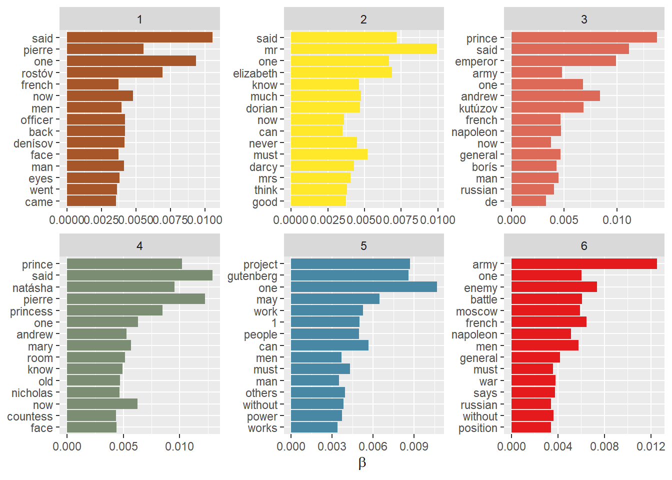
Let’s look at the words with the highest probabilities to below to each of the 6 topics. There are clearly some words from each book that are more salient in some topics. Let’s get serious and use all the model results.
library(tidytext)
library(tidyverse)
library(topicmodels)
library(scales)
library(broom)

# Plot
42broom::tidy(shuffle_lda, matrix = "beta") |>
  dplyr::group_by(topic) |>
  dplyr::slice_max(order_by = beta, n = 15) |>
  ggplot(aes(x= term |> reorder(beta), y= beta, fill=topic)) +
  geom_col() +
  coord_flip()+
  scale_fill_distiller(palette="Set1")+
  facet_wrap(~topic, scales = "free") +
  labs(x = NULL, y = expression(beta))+
theme(legend.position = "none")- 42
- Extract the \(\beta\) probabilities from the model, word-topic probabilities.
Working with word-topic (\(\beta\)) and topic-book (\(\gamma\)) probabilities
\(\beta\) controls the distribution of words within a topic. It is a Dirichlet prior on the per-topic word distributions. In other words, it represents the probability of a specific word being present in a topic. A higher beta value will result in a more diverse set of words within a topic, while a lower beta value will lead to a more focused set of words.
\(\gamma\) controls the distribution of topics within a document. It is a Dirichlet prior on the per-document topic distributions. It governs the probability of a specific topic being present in a document. A higher gamma value will result in a more diverse set of topics within a document, while a lower gamma value will lead to a more focused set of topics.
We extract model results in tidy format using the broom package tidy() function, which extracts model results in our favourite format. Let’s look in detail at model results for both key parameters.
library(tidytext)
library(tidyverse)
library(topicmodels)
library(scales)

# Beta ####
43words_beta <- broom::tidy(shuffle_lda, matrix = "beta")

# Gamma ####
44chapters_gamma <- broom::tidy(shuffle_lda, matrix = "gamma")

# Plot
broom::tidy(shuffle_lda, matrix = "gamma") |>
45  tidyr::separate(document, c("title", "chapter"), sep = "_", convert = TRUE) |>
  dplyr::mutate(title = reorder(title, gamma * topic)) %>%
  ggplot(aes(factor(topic), gamma, color=title)) +
  geom_boxplot() +
  facet_wrap(~title) +
  labs(x = "topic", y = expression(gamma))+
theme(legend.position = "none")- 43
- \(\beta\) probabilities: Word within a Topic
- 44
- \(\gamma\) probabilities: Topics within a Chapter
- 45
-
Break apart a variable using
separate()function
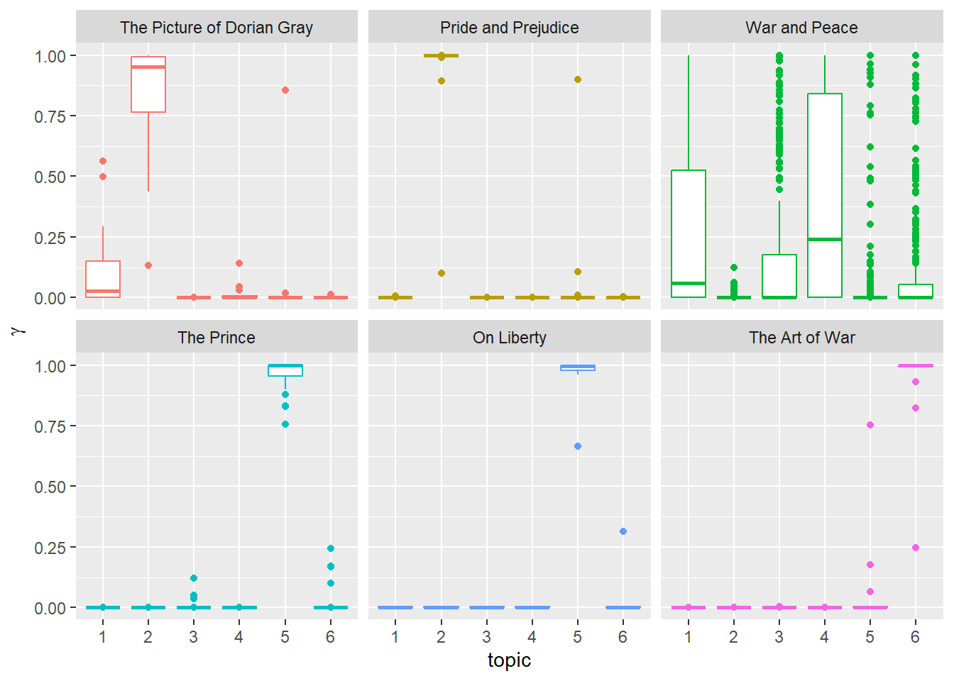
We can see that \(\gamma\) worked well for some books, not so much for others.
Let’s look more closely at the classification –where it succeeded and where it failed.
Did it work?
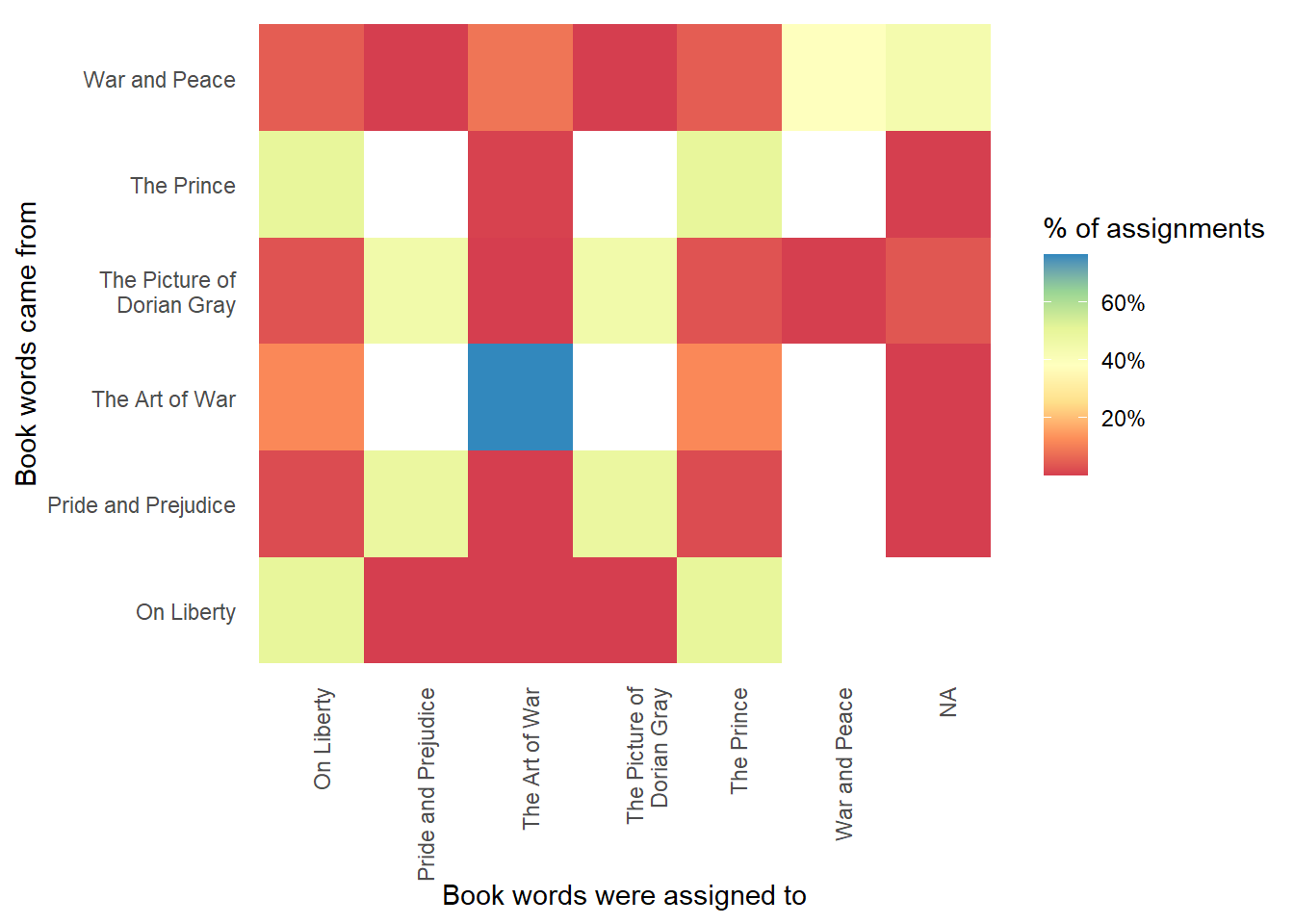
To know how well the topic classification worked, we build a tile grid to relate how many chapters from each book were correctly classified into the book they originated from.
Now the picture is clearer. Some books, the shortest and distinct from the others, were for the most part correctly classified.
To get better results from this approach we need to delve deeper into the tuning parameters of the model or try an entirely different text-data approach.
library(tidytext)
library(tidyverse)
library(topicmodels)
library(scales)

# Save chapter classifications ####
chapter_classifications <- broom::tidy(shuffle_lda, matrix = "gamma") |>
  tidyr::separate(document, c("title", "chapter"), sep = "_", convert = TRUE)  %>%
  dplyr::group_by(title, chapter) %>%
  dplyr::slice_max(gamma) %>%
  dplyr::ungroup()

# Save most likely topics for each book ####
46book_topics <- chapter_classifications %>%
  dplyr::count(title, topic) %>%
  dplyr::group_by(title) %>%
  dplyr::slice_max(n, n = 1) %>%
  dplyr::ungroup() %>%
  dplyr::transmute(consensus = title, topic)

# Join the results ####
47chapter_classifications %>%
  dplyr::left_join(book_topics, by = "topic") %>%
  dplyr::filter(title != consensus)

# Add Document Term Matrix data to results and join book classifications ####
assignments <- broom::augment(shuffle_lda, data = shuffle_dtm) |>
  tidyr::separate(document, c("title", "chapter"),
           sep = "_", convert = TRUE) %>%
  dplyr::left_join(book_topics, by = c(".topic" = "topic"))

# Visualise the result ####
assignments %>%
  dplyr::count(title, consensus, wt = count) %>%
48  dplyr::mutate(across(c(title, consensus), ~str_wrap(., 20))) %>%
  dplyr::group_by(title) %>%
  dplyr::mutate(percent = n / sum(n)) %>%
  ggplot(aes(consensus, title, fill = percent)) +
  geom_tile() +
  scale_fill_distiller(palette = "Spectral", direction=1,label = percent_format()) +
  theme_minimal() +
  theme(axis.text.x = element_text(angle = 90, hjust = 1),
        panel.grid = element_blank()) +
  labs(x = "Book words were assigned to",
       y = "Book words came from",
fill = "% of assignments")- 46
- Save the most-likely result as a consensus variable
- 47
- Join the consensus result to the data
- 48
-
Notice
across()which facilitates applying a function to multiple columns
# A tibble: 237 × 5
   title      chapter topic gamma consensus
   <chr>        <int> <int> <dbl> <chr>
 1 On Liberty       1     5 0.955 The Prince
 2 On Liberty       2     5 0.629 The Prince
 3 On Liberty       3     5 0.974 The Prince
 4 On Liberty       4     5 0.607 The Prince
 5 On Liberty       5     5 0.993 The Prince
 6 On Liberty       6     5 1.000 The Prince
 7 On Liberty       7     5 1.000 The Prince
 8 On Liberty       8     5 1.000 The Prince
 9 On Liberty       9     5 1.000 The Prince
10 On Liberty      10     5 1.000 The Prince
# ℹ 227 more rows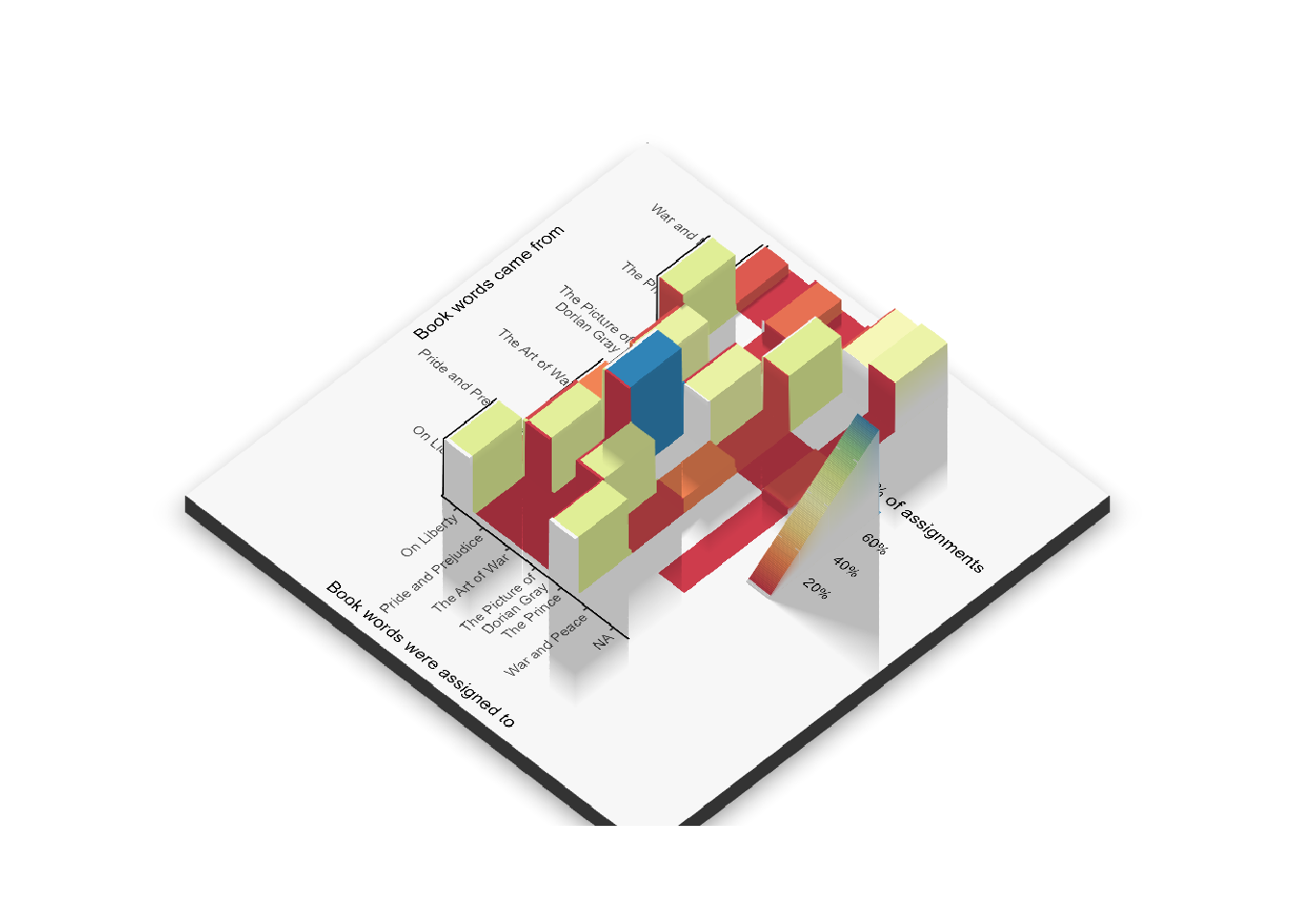
Bonus track: Networks of n-grams in the work of David Hume
There are many types of relational analysis you can do with text. An interesting one is how expressions, measured as n-grams (adjacent words), are related to one another using networks. We’ll use David Hume’s An Enquiry Concerning Human Understanding to illustrate, which we will import from Project Gutenberg.
We will tokenize differently using the n-grams output option in the unnest_tokens() function. We need to decide how many adjacent words will be tokenized, so for ease we will do pairs of words.
After we tokenize and count, we need to turn each pair of words into a network, which is easy using the igraph package and then well use the ggraph package to visualise it. Networks are made of nodes and edges, and in this case an n-gram of two words means two nodes are connected to each other by an edge. Using the graph_from_data_frame() function, we can turn a tibble made of pairs of words into a network.
Tip
ggraph vignette
Take a look at the vignette for this package here
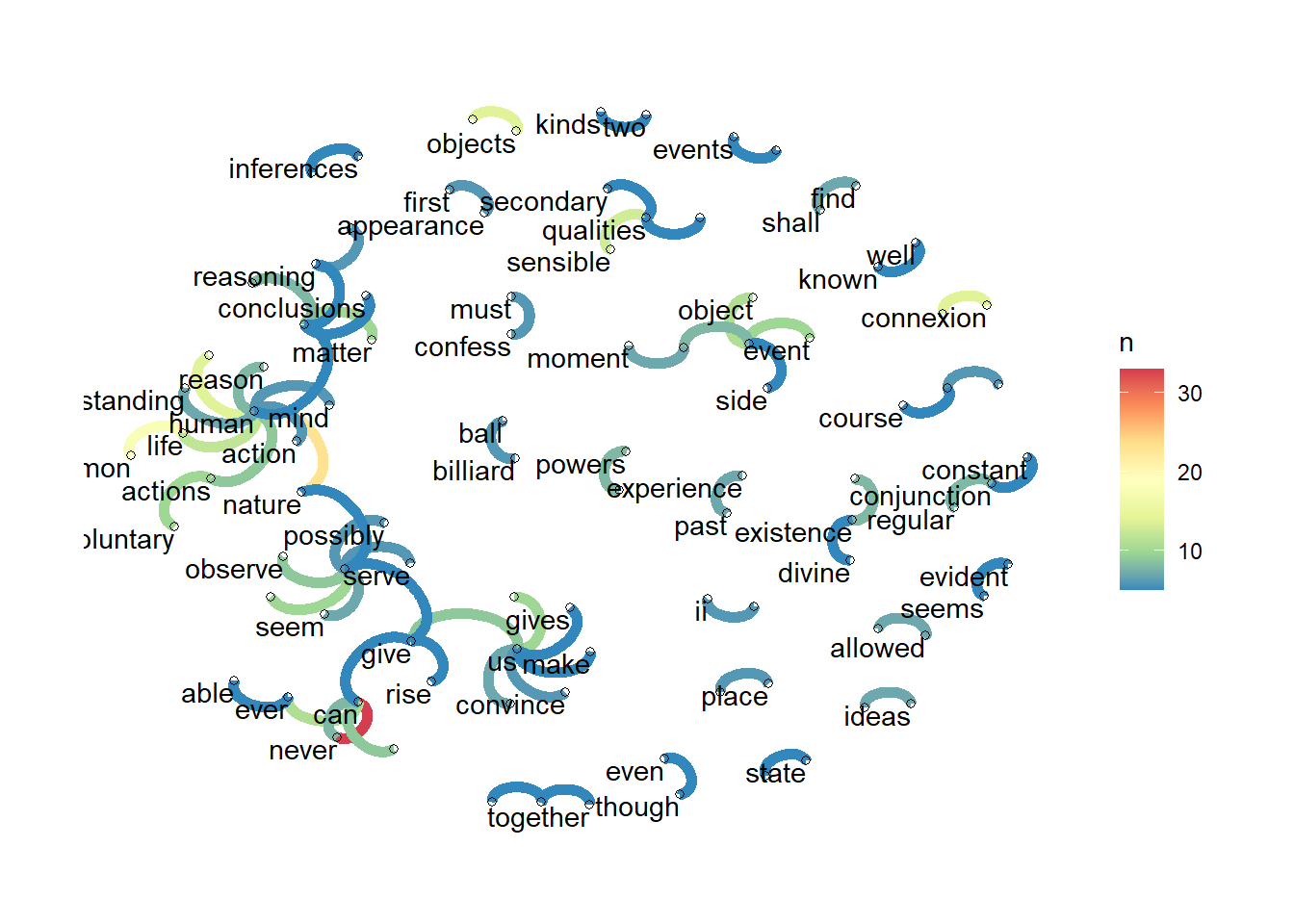
Look at the code below that shows all the steps, from tokenizing to plotting the network. Notice the changes in ggraph, like the layout (an algorithm that places nodes in the graph according to their properties) and the geoms –for both edges and nodes.
But also look at the results. The n-grams show relationships between key concepts in this important work on epistemology, like natural events, or how reasoning is connected to observation, the mind and matter.
library(ggraph)     # ggplot2 tools for networks
library(tidygraph)  # Tidy objects for networks
library(igraph)     # the workhorse for network analysis in R
library(gutenbergr) # To import books from Project Gutenberg
library(tidytext)
library(tidyverse)
library(RColorBrewer)
library(viridis)

gutenbergr::gutenberg_download(gutenberg_id = 9662, mirror = "http://mirrors.xmission.com/gutenberg/") |>
  tibble::as_tibble() |>
49  tidytext::unnest_tokens(
    input = "text",
    output = "ngrams",
    n=2,
    token = "ngrams",
    to_lower = TRUE) |>
50  tidyr::separate(ngrams, into = rep(paste0("word_",1:2), sep = " ")) |>
51  dplyr::filter(!word_1 %in% stopwords::stopwords(language = "en"),
                !word_2 %in% stopwords::stopwords(language = "en")) |>
  dplyr::filter(nchar(word_1) > 1,nchar(word_2) > 1) |>
52  dplyr::count(word_1,word_2,sort = TRUE) |>
  dplyr::slice_max(order_by = n, n=50) |>
53  igraph::graph_from_data_frame() |>
54  ggraph::ggraph(layout="fr")+
55  ggraph::geom_edge_arc(aes(edge_color=n), edge_width = 2)+
56  ggraph::geom_node_point(shape=1)+
  ggraph::geom_node_text(aes(label = name), vjust = 1, hjust = 1,  check_overlap = TRUE)+
57  ggraph::scale_edge_color_distiller(palette="Spectral")+
theme_graph()- 49
- We now create n-grams of length 2, all combinations of 2 consecutive words
- 50
- Separate the n-grams to remove stopwords
- 51
- Remove all stopwords and single-letter words
- 52
- Count and keep most frequent n-grams
- 53
-
Turn data frame into igraph object to build a network using the
graph_from_data_frame()function - 54
- Use ggraph with specified layout
- 55
- Graph the edges or links
- 56
- Graph the nodes and labels them
- 57
- Clean up with theme made for networks and put a color scale on the connections
🏗 Practice 3: Project Gutenberg
The core tokenise-count-plot loop runs right here in your browser on Jane Austen’s novels; the Gutenberg downloads wait for your own R session.
Key takeaways
- Text becomes data the moment you tokenise it into one row per unit (word, ngram, sentence).
- Stopword removal, stemming and lemmatising all reduce noise before you count anything.
- Sentiment lexicons disagree with each other – always check more than one before trusting a result.
- Topic modelling finds latent structure in a corpus without you labelling anything by hand.
- Wrapping a repeated analysis in a function (like
book_sentiments()) is what makes it reusable across books.
Footnotes
Saif M. Mohammad and Peter Turney (2013) Crowdsourcing a Word-Emotion Association Lexicon. Computational Intelligence, 29(3): 436-465.↩︎
Section based on Chapter 6 of “Text Mining with R: A Tidy Approach”↩︎
Confused about LDA and topic modelling? Confusion is the first step to understanding, so explore this topic-modelling walkthrough↩︎
Citation
BibTeX citation:
@online{amaya2022,
  author = {Amaya, Nelson},
  title = {Data from Words 📚},
  date = {2022-07-31},
  url = {https://r4dev.netlify.app/sessions_workshop/03-text/03-text},
  langid = {en}
}
For attribution, please cite this work as:
Amaya, Nelson. 2022. “Data from Words 📚.” July 31. https://r4dev.netlify.app/sessions_workshop/03-text/03-text.