Just take it 🌏

Learn how to scrape information from websites

Sometimes you need to bring data straight from a website. Scrape IMDb movie rankings, U2 lyrics and untranslatable words.

If it doesn’t exist on the internet, it doesn’t exist.
–Kenneth Goldsmith

PART I: Pick it, grab it

Although you’ve learned to use API and dedicated packages to get information from online sources, sometimes you want to just take a table from Wikipedia, or some text from a webpage and bring it into R.

To do this you need two tools:

1. The rvest package, which helps read HTML pages and gather information from them
2. Install the Selector Gadget Extension in your browser. This will help you select the object you want to import.

TipI’ll say it again: Read package vignettes

Check out the rvest vignette

How does the Selector Gadget work? By clicking in an HTML page until the objects you want are selected in green.

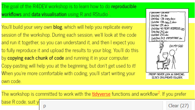
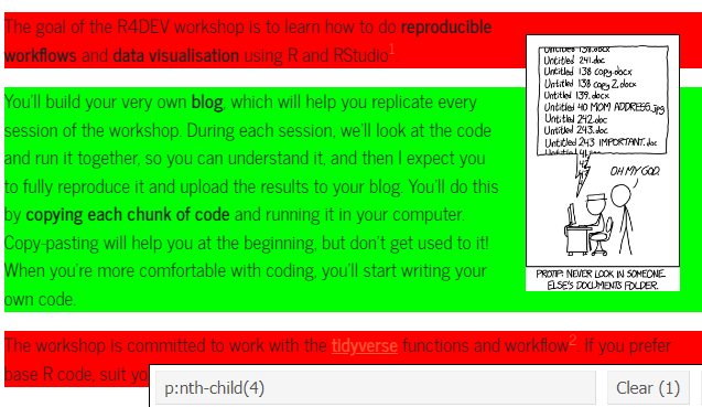
Imagine you want to extract text from the Home page of R4DEV, but you only want one paragraph. Clicking the elements you want until only what you want is highlighted in green, as shown below, will let you know which element you’ll scrap. The selected element p:nth-child(4) will appear below and you can copy it to use it as it is shown below.

Selecting some elements

When green, you got it!

Top movies according to IMDb

IMDb has a list of the best ranked movies. We’ll pull it straight from the website using rvest. Using the Selector Gadget, we click on the objects of the webpage we want and bring them to the code that will pull that information and transform it into text.

We will extract the ranking, title, year and country of every movie from the Wikipedia entry.

For tables, rvest has a shortcut that spares you the click-hunting: html_table() grabs an HTML table and returns it as a tibble directly. Whenever what you want looks like a table on the page, reach for it first –hand-picked selectors like the ones above are brittle, and break whenever the page structure changes (this very session broke that way once; ask the instructor).

library(tidyverse)
library(rvest)

imdb_top_url <- "https://fr.wikipedia.org/wiki/Top_250_de_l%27Internet_Movie_Database"

# Scrape ! ####
imdb_top_250_raw <- imdb_top_url |>
  rvest::read_html() |>
  rvest::html_element("table.wikitable") |>
  rvest::html_table()

imdb_top_250_raw

1

Save the URL of the page we want

2

Start the pipe with the URL

3

Read the page as HTML with read_html()

4

Select the first element with class wikitable –Wikipedia uses that class for its data tables. Selector Gadget confirms it in one click

5

html_table() parses the rows and columns straight into a tibble –no text-wrangling gymnastics needed

# A tibble: 250 × 6
    Rang `Titre français`     `Titre original` `Réalisateur(s)` Année `Pays[10]`
   <int> <chr>                <chr>            <chr>            <int> <chr>     
 1     1 Les Évadés           The Shawshank R… Frank Darabont    1994 États-Unis
 2     2 Le Parrain           The Godfather    Francis Ford Co…  1972 États-Unis
 3     3 Le Parrain, 2e part… The Godfather: … Francis Ford Co…  1974 États-Unis
 4     4 Pulp Fiction         Pulp Fiction     Quentin Taranti…  1994 États-Unis
 5     5 Le Bon, la Brute et… Il buono, il br… Sergio Leone      1966 Italie    
 6     6 The Dark Knight : L… The Dark Knight  Christopher Nol…  2008 États-Unis
 7     7 Douze Hommes en col… 12 Angry Men     Sidney Lumet      1957 États-Unis
 8     8 La Liste de Schindl… Schindler's List Steven Spielberg  1993 États-Unis
 9     9 Le Seigneur des ann… The Lord of the… Peter Jackson     2003 États-Unis
10    10 Fight Club           Fight Club       David Fincher     1999 États-Unis
# ℹ 240 more rows

TipA little HTML is enough

Learn a little HTML, it will help you identify quickly the information you want to retrieve from a website. Read the Get Started section in rvest.

Now a little cleaning –scraped column names arrive messy and accented– and we create a searchable table using reactable, which should be your go-to package for interactive tables.

library(tidyverse)
library(RColorBrewer)
library(reactable)
library(reactablefmtr)

imdb_top_250_raw |>
  janitor::clean_names() |>
  dplyr::select(rank = rang, title = titre_original, year = annee, country = starts_with("pays")) |>
  dplyr::mutate(across(c(rank, year), as.numeric)) |>
  # Table
  reactable(
    filterable = TRUE,
    searchable = TRUE,
    highlight = TRUE,
    striped = TRUE,
    resizable = TRUE,
    theme = journal(font_size=12)
    )

6

Start with the scraped table

7

clean_names() from janitor turns Titre français and friends into safe lowercase names without accents

8

We keep and rename the columns we care about –starts_with("pays") catches the country column even though Wikipedia decorates its name with a footnote marker

9

We change rank and year to numeric values using across(), which is used to modify multiple columns

Rejoinder: Feeling U2

Now that we know how to get data from websites, carry out text analysis and visualise, let’s put together all three to something concrete: doing sentiment analysis of all U2 lyrics.

First, we get all lyrics from U2, which are collected in their website. We go to the lyrics page and retrieve the URL of each song. There are over 240 lyrics, but the URLs for each one are not sequential, and include random large numbers. So after extracting the element we want using html_elements(), we use the html_attr() function to retrieve the URL for each lyric. Then we can pass all URLs through a loop and save into an empty list, as we did with songs before.

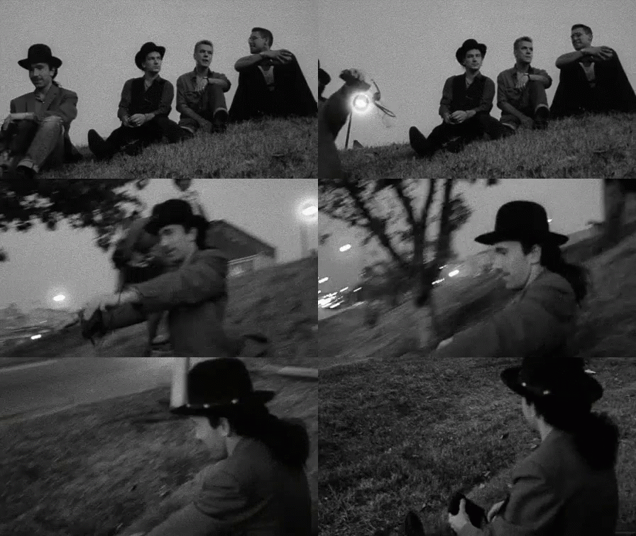
The Edge

library(tidyverse)
library(rvest)
library(tidytext)

# Extract all song lyrics URLs ####
u2_urls <- "https://www.u2.com/music/lyrics" |>
  # First step as before
  rvest::read_html() |>
  # We select the element we want, which is the link to every song
  rvest::html_elements(".lyricItem--link") |>
  # We extract the link to each song by picking an attribute, which for links is href
  rvest::html_attr("href") |>
  tibble::as_tibble() |>
  # We keep only one variable which is the URL of each song
  dplyr::transmute(url = str_c("https://www.u2.com",value))

# Create an empty list and save all song lyrics using a loop ###
u2_lyrics <- list()
for(i in u2_urls$url) {

  u2_lyrics[[i]] <- rvest::read_html(i) |>
    # Extract what we want
    rvest::html_elements("p") |>
    # Make it into text using html_text2
    rvest::html_text2() |>
    as_tibble() 
    
}

TipScrape once, save, reuse

The loop above knocks on u2.com about 240 times and takes several minutes –running it on every render would be slow and rude to the band’s web server. So we practice what session 2 preached: we ran it once, saved the result, and load the snapshot from now on. split() rebuilds the exact same named list the loop produced.

library(tidyverse)

u2_lyrics_df <- readr::read_csv(paste0(getwd(), "/u2_lyrics.csv"))

u2_lyrics <- split(dplyr::select(u2_lyrics_df, value), u2_lyrics_df$url)

Second, we do a little wrangling to transform the list to a tibble, our favorite layout and format for rectangular datasets. We use imap() to name each element in the list, and then map_df() to bind them all together. This leaves us with a dataset where each row includes the lyrics of a song.

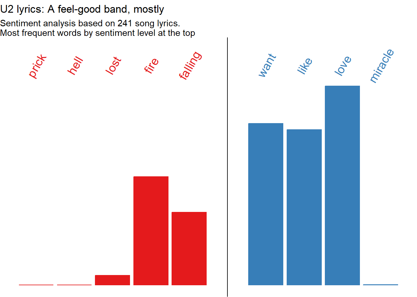
Third, we tokenise by words, remove stopwords and join the sentiment lexicon. Just as we did with books before. With a twist: we’ll use both words and n-grams as tokens. For words, we calculate the frequency for each value of the sentiment lexicon, and feed into ggplot. For flair, we add the most frequent word for each sentiment value at the top of the graph and plot the frequency of all words lyrics. For ngrams, we just count the expressions that are more frequent in the entire lyrics space.

Token: Using sindle words

library(tidyverse)
library(tidytext)

u2_lyrics |>
  # Add a variable inside of every tibble in the list with the url, using imap
  purrr::imap(~mutate(.x, url=.y)) |>
  # Bind into a data frame all lyrics
  purrr::map_df(bind_rows) |>
  dplyr::filter(!str_detect(value,"No lyrics")) |>
  # Unnest words
  tidytext::unnest_tokens(input = "value", output = "text", token = "words") |>
  # Remove stopwords
  dplyr::anti_join(stopwords::stopwords("en") |> as_tibble(), by=c("text"="value")) |>
  # Join sentiment lexicon
  dplyr::inner_join(tidytext::get_sentiments("afinn"), by=c("text"="word")) |>
  # Calculate most frequent word by sentiment lexicon
  dplyr::group_by(text) |>
  dplyr::mutate(word_freq = n()) |>
  dplyr::ungroup() |>
  # Summarise ####
  dplyr::group_by(value) |>
  dplyr::mutate(n = n(),
                p = n/sum(n),
                c = case_when(value<0 ~ "Negative",
                              value==0 ~ "Neutral",
                              value>0 ~ "Positive") |>
                  factor()) |>
  # Feed to ggplot
  ggplot(aes(x=value,y=n,fill=c, color=c))+
  geom_col()+
  # Notice how the data is filtered inside of the geom ####
  geom_text(data = . %>%
              dplyr::group_by(value) %>%
              dplyr::slice_max(n=1, order_by = word_freq) %>%
              dplyr::distinct(text, .keep_all = TRUE),
             aes(y=700000, label=text), 
            angle=60, size=5)+
  geom_vline(xintercept = 0)+
  scale_x_continuous(breaks=seq(from=-5,to=5,by=1))+
  scale_y_continuous(limits = c(0, 750000))+
  scale_fill_brewer(palette = "Set1")+
  scale_color_brewer(palette = "Set1")+
  labs(title = "U2 lyrics: A feel-good band, mostly",
       subtitle = "Sentiment analysis based on 241 song lyrics.\nMost frequent words by sentiment level at the top",
    x="Sentiment lexicon: AFINN",
    y= "Word frequency")+
  theme_void()+
  theme(legend.position = "none")

Token: Using a 3-word n-gram

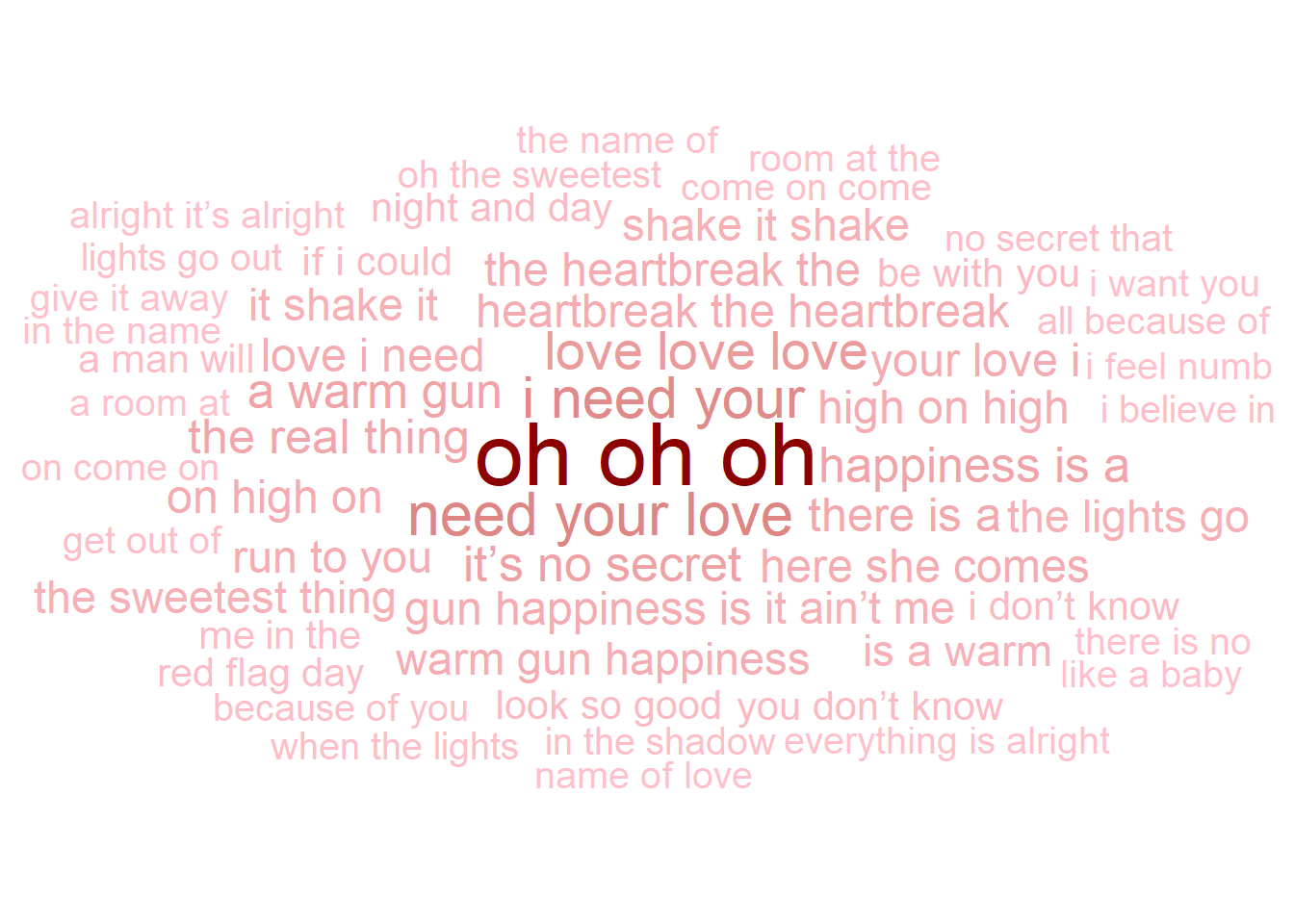
library(tidyverse)
library(tidytext)
library(ggwordcloud)

u2_lyrics |>
  # Identify each list with the url using imap
  purrr::imap(~mutate(.x, url=.y)) |>
  # Bind into a data frame all lyrics
  purrr::map_df(bind_rows) |>
  dplyr::filter(!str_detect(value,"No lyrics")) |>
  # Unnest 
  tidytext::unnest_tokens(input = "value", output = "ngram", token = "ngrams", n=3) |>
  dplyr::count(ngram, sort=TRUE) |>
  dplyr::distinct_all() |>
  dplyr::slice_max(order_by = n, n = 50) |>
  ggplot()+
  ggwordcloud::geom_text_wordcloud(aes(label = ngram, size = n, color=n)) +
  scale_size_area(max_size = 12) + 
  scale_color_gradient(low = "pink", high = "red4")+
  theme_minimal()

TipMore ggplot2 extensions

You now know how to work with ggplot2 and some extensions like ggridges or ggiraph. But there are many more you might want to check out. The gallery of over a hundred extensions is here, and some of my favorites are listed below:

• ggdist provides stats and geoms for visualizing distributions and uncertainty.
• ggExtra lets you add marginal density plots or histograms to ggplot2 scatterplots.
• ggpattern includes pattern fills for geoms.
• ggcorrplot enables correlation matrix plots
• hrbrthemes nice themes
• ggdag for causal inference fans: Directed Acyclical Graphs (DAGs).
• ggmapinset zoom into parts of sf maps.

Eunoia, words that don’t translate¹

This site holds words and concepts in multiple languages that don’t translate. Getting all the words and definitions is not easy, as each time you enter the site, a random set of words pops up. There is no easy way to download the list of words, but we can still do it.

Exactly

How many words are there, how can we scrap them? As of late 2021, there were over 500. In 2023, that number grew even more, to over 700.

We are doing this task by throwing computational brute force: we will scrape the site multiple times until no new words are retrieved, using while function that will run until no new words are found.

The code takes time to run, but it does the trick.

library(rvest)
library(tidyverse)

# URL  ####
eunoia_url <- "https://eunoia.world/"

# Step 1 - Create an empty list and an empty data frame. We will store the results there ####
eunoia <- list()
eunoia_df <- tibble()

# Step 2 - We'll use while function to scrap the website until we have 700 different words ####
while (tally(eunoia_df) <= 690) {
  
  # i) Loop 100 scraps of the website and save them into the empty list
  for (i in c(1:100)) {
  
  # A - Start with empty list and double bracket to save as elements
  eunoia[[i]] <- eunoia_url |>
    rvest::read_html() |>
    rvest::html_elements("td:nth-child(3) , td:nth-child(2) , td:nth-child(1)") |>
    rvest::html_text() |>
    tibble::as_tibble() |>
    dplyr::mutate(names = rep(c("word","description","language"), times = n()/3)) |>
    tidyr::pivot_wider(values_from = value, names_from = names, values_fn = list) |> 
    tidyr::unnest(cols = everything())
  
  # B - Put together all the results into a data frame using map_df and removing repeated words
  eunoia_df <- eunoia |>
    purrr::map_df(bind_rows) |>
    dplyr::distinct_all()
  
  }
}

Now let’s check all the downloaded untranslatable words is a reactable table, using a bootswatch theme and aggregating all words by language groups using groupBy() and a bit of column styling.

Tipreactable tables can be very fancy

You can customise these tables a lot. Check out these examples and re-use any elements that you want to style the tables.

library(tidyverse)
library(reactable)
library(reactablefmtr)

eunoia_scraped |>
  dplyr::select(1:3) |>
  dplyr::mutate(language=factor(language)) |>
  reactable(
    filterable = TRUE, 
    searchable = TRUE, 
    highlight = TRUE, 
    striped = TRUE, 
    resizable = TRUE,
    theme = cerulean(),
    groupBy = "language",
    columns = list(
     word = colDef(
      html = TRUE,
      style = list(fontWeight = "bold")
    ),
    description = colDef(
      html = TRUE,
      style = list(fontStyle = "italic")
    )
      )
  )

PART II: Beyond static websites

Everything so far assumed the data is already in the page: read_html() downloads the HTML the server sends, and we harvest it. But many modern websites arrive almost empty and build their content afterwards, by running JavaScript in your browser. read_html() never runs JavaScript, so it sees only the hollow shell.

See it for yourself. quotes.toscrape.com is a sandbox built for practicing scraping, and it serves the same quotes twice: once as normal HTML, and once rendered by JavaScript at /js/. Watch what happens when we scrape the JavaScript version the old way:

library(tidyverse)
library(rvest)

rvest::read_html("https://quotes.toscrape.com/js/") |>
  rvest::html_elements(".quote .text") |>
  rvest::html_text2()

11

The same selectors that work on the static version return… nothing. The quotes aren’t in the HTML the server sent –they are built by JavaScript after the page loads.

character(0)

The fix is one function swap: read_html_live() opens a real (but invisible) Chrome window using the chromote package, lets the JavaScript run, and then hands the rendered page to the exact same selector functions you already know.

quotes_live <- rvest::read_html_live("https://quotes.toscrape.com/js/")

quotes_live |>
  rvest::html_elements(".quote") |>
  purrr::map_df(\(q) tibble(
    quote  = q |> html_element(".text") |> html_text2(),
    author = q |> html_element(".author") |> html_text2()
  ))

12

read_html_live() needs the chromote package and a Chrome-based browser installed –that’s it. No Java, no Docker, no drivers.

13

From here on, everything is the rvest you already know: same selectors, same functions.

14

A little map_df() pattern to turn each quote <div> into a row –one anonymous function, one tidy tibble.

# A tibble: 10 × 2
   quote                                                                  author
   <chr>                                                                  <chr> 
 1 “The world as we have created it is a process of our thinking. It can… Alber…
 2 “It is our choices, Harry, that show what we truly are, far more than… J.K. …
 3 “There are only two ways to live your life. One is as though nothing … Alber…
 4 “The person, be it gentleman or lady, who has not pleasure in a good … Jane …
 5 “Imperfection is beauty, madness is genius and it's better to be abso… Maril…
 6 “Try not to become a man of success. Rather become a man of value.”    Alber…
 7 “It is better to be hated for what you are than to be loved for what … André…
 8 “I have not failed. I've just found 10,000 ways that won't work.”      Thoma…
 9 “A woman is like a tea bag; you never know how strong it is until it'… Elean…
10 “A day without sunshine is like, you know, night.”                     Steve…

TipNeed to click, type or scroll?

read_html_live() covers the most common case: pages that render with JavaScript. When you also need to interact –click “load more”, fill a search box, log in– use selenider: it drives the same headless Chrome with a friendly syntax (open_url(), s(".button") |> elem_click()).

You may find old tutorials using RSelenium for this. It works, but it is a heavyweight from another era –it needs Java and browser drivers, and its maintenance has wound down. chromote and selenider are its modern replacements.

🏗 Practice 6: Scrape

NoteEasy

• Find a website with info you want to bring to R
• Visualise the data (plot, map, etc.)
• Scrape any Wikipedia table and plot the result in R
• Scrape all ten quotes from the JavaScript sandbox with read_html_live(), including the tags of each quote

ImportantIntermediate

• Scrape the lyrics for Bob Dylan, Pearl Jam or another artist you can find online. Re-create the sentiment analysis workflow for their lyrics.
• The U2 page with lyrics also shows every time each song has been played during a tour since the late 80s. Scrap the tour dates and visualise song popularity through time.

Footnotes

1. Thanks to Zélie for finding this amazing site.