Think Bayes 🤔

A very short introduction to bayesian updating

Toss a globe, count the water, and watch a probability distribution learn. A gentle first contact with Bayesian inference, animated with the tools from session 4.

“It appears to be a quite general principle that, whenever there is a randomized way of doing something, then there is a nonrandomized way that delivers better performance but requires more thought.”
–E.T. Jaynes

Part I: Why Bayes?

Every statistics course you took taught you to ask: how surprising is my data, assuming some hypothesis is true? Bayesian analysis asks the question you actually care about, in the direction you actually care about: given the data I saw, what should I now believe?

The machinery is one line –Bayes’ theorem– and one discipline: beliefs are distributions, not numbers, and data doesn’t replace them, it updates them.

What proportion of the Earth is water?

The classic teaching example, from Richard McElreath’s Statistical Rethinking¹: toss an inflatable globe in the air, catch it, and write down whether your index finger landed on Water or Land. Each toss is a noisy observation of one number: \(p\), the true proportion of the Earth covered by water (about 0.71, but pretend you don’t know).

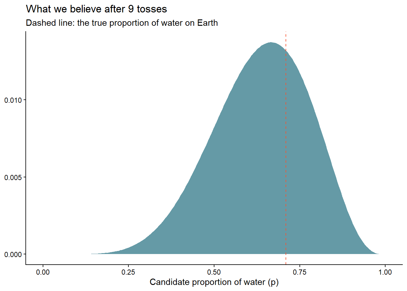
Nine tosses give us W L W W W L W L W –six waters. What should we believe about \(p\)? We compute it with a grid approximation: try every candidate value of \(p\), score how well each explains the data, and weigh by what we believed before.

library(tidyverse)

1tosses <- c("W","L","W","W","W","L","W","L","W")

2globe_posterior <- tibble(p = seq(0, 1, length.out = 200)) |>
  dplyr::mutate(
3    prior      = 1,
4    likelihood = dbinom(sum(tosses == "W"), size = length(tosses), prob = p),
5    posterior  = likelihood * prior / sum(likelihood * prior)
  )

globe_posterior |>
  ggplot(aes(x = p, y = posterior)) +
  geom_area(fill = "#226F7F", alpha = 0.7) +
6  geom_vline(xintercept = 0.71, linetype = "dashed", color = "#F75431") +
  labs(title = "What we believe after 9 tosses",
       subtitle = "Dashed line: the true proportion of water on Earth",
       x = "Candidate proportion of water (p)", y = NULL) +
  theme_classic()

1

Our data: nine catches, six fingers on water.

2

The “grid”: 200 candidate values for \(p\) between 0 (all land) and 1 (all water).

3

A flat prior: before tossing, we pretend every proportion is equally plausible. Priors can –and usually should– know more than this.

4

The likelihood: for each candidate \(p\), the probability of seeing 6 waters in 9 tosses. Plain old dbinom() –you have used it since session 4’s coin flips.

5

Bayes’ theorem, literally typed out: posterior ∝ likelihood × prior. The division just makes it sum to one.

6

We never told the code the answer –look where the belief piles up anyway.

Watch the learning happen

A posterior is not a verdict, it is a running belief –so let’s animate it updating toss by toss, with the exact gganimate tools from session 4. Frame \(n\) shows what we believe after the first \(n\) tosses:

library(gganimate)

7update_frames <- purrr::map_df(0:length(tosses), \(n) {
  tibble(p = seq(0, 1, length.out = 200)) |>
    dplyr::mutate(
      posterior = dbinom(sum(tosses[seq_len(n)] == "W"), size = n, prob = p),
      posterior = posterior / sum(posterior),
      n_tosses  = n,
      label     = ifelse(n == 0, "Before any data (the prior)",
                         paste0("After ", n, " tosses: ", paste(tosses[seq_len(n)], collapse = " ")))
    )
})

update_frames |>
  ggplot(aes(x = p, y = posterior)) +
  geom_area(fill = "#226F7F", alpha = 0.7) +
  geom_vline(xintercept = 0.71, linetype = "dashed", color = "#F75431") +
8  labs(title = "{closest_state}",
       x = "Proportion of water (p)", y = NULL) +
  theme_classic() +
  gganimate::transition_states(label, transition_length = 2, state_length = 3, wrap = FALSE) +
  gganimate::ease_aes("cubic-in-out")

7

For each \(n\) from 0 to 9, we recompute the posterior using only the first \(n\) tosses –ten snapshots of a mind changing.

8

transition_states() from session 4, nothing new. Watch how the first W rules out \(p = 0\) completely, and how each toss reshapes –but never erases– what came before.

Bayesian updating, one toss at a time

Part II: Your turn to believe

The window below runs R in your browser. Change the prior –make it stubborn (p^10), skeptical of water ((1-p)^3), or opinionated like a geographer (dbeta(p, 7, 3))– and watch how much (or little) the same 9 tosses can teach different minds.

TipPlay more

This repo ships a small Shiny simulator with sliders for the prior and the data –break your intuitions at will. It’s live below, or run it yourself with shiny::runApp("shiny/BayesApp") from the project.

Where next

This was the whole idea of Bayes in one session; the rest is craft. When you are ready:

• Statistical Rethinking (McElreath) –start here, no contest. R code for everything.
• Bayes Rules! –free online, gentler on-ramp, tidyverse throughout.
• brms –when you want real models: multilevel regression with lm()-like syntax, Stan under the hood.
• bayesplot –diagnostics and posterior visualisations that match what you learned in session 2.

🏗 Practice 13: Update yourself

NoteEasy

• Re-run the grid approximation with 100 tosses (72 W). What happened to the width of the posterior? Why?
• In the browser window above, find a prior strong enough that 9 tosses barely move it. How much data does it take to overwhelm it?

ImportantIntermediate

• Animate the 100-toss updating. At what point does the animation get boring? That boredom has a name: convergence
• The globe example has one parameter. Write down –just on paper– what the grid would look like for two parameters. Now you know why MCMC exists

Footnotes

1. The best statistics book you will ever read, and the source of this example. The lectures are free on YouTube.